Mobile Robot Control 2023 Group 4

Group members:
| Name | student ID |
|---|---|
| Lowe Blom | 1266020 |
| Rainier Heijne | 1227575 |
| Tom Minten | 1372300 |
Exercise 1: Don't crash (video link):
https://drive.google.com/file/d/1zgMMQwU3ZrADZJuFCLglQiefVecF3_95/view?usp=sharing
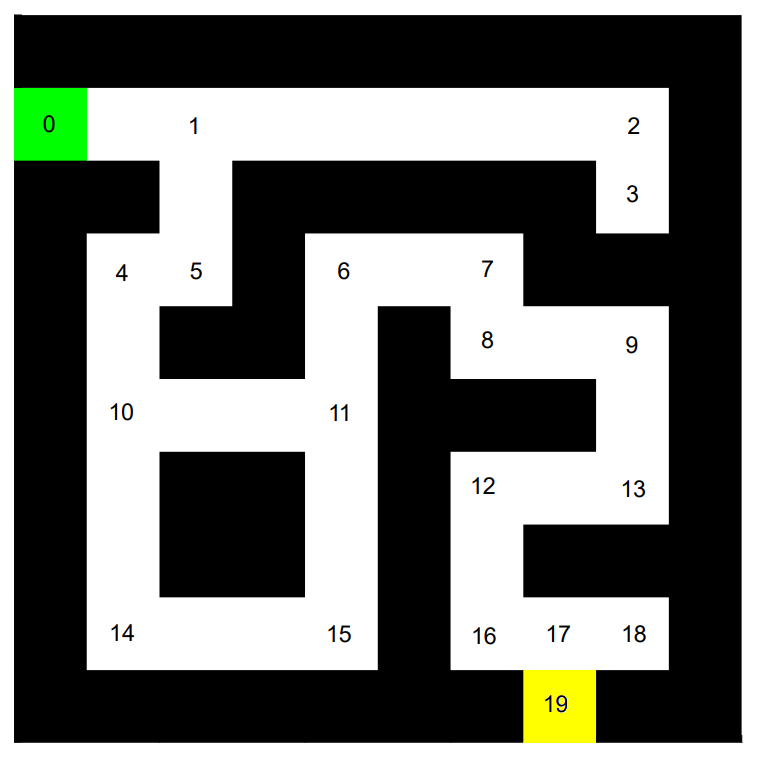
Exercise 2: A* algorithm
- The code can be found on our gitlab page
- The middle nodes in a straight line without more than two neighbors can be removed. Since the speed of the algorithm is O(n) with n the size of the grid, removing cells from the grid will improve the performance of the algorithm.

The robot has to drive 5 meters through a corridor with a width of 1 to 2 meters, without a collision with present obstacles. Our solution is based on looking for free space around and between objects. The following steps are taken for each laser data set:
1. Laser sensor data is read to detect obstacles.
2. Detected obstacles are stored in a list of objects with all the relative positions of the scan points of each object.
3. The code identifies the boundaries of the each detected object.
4. If there are at least two detected objects, the code finds the shortest distance with a minimum width between neighboring obstacles.
5. The target point is set as the middle point of the largest gap between all objects

6. Based on the target point's position, the robot's linear and angular velocities are set
7. If no suitable distance is found or only one object is detected, the robot drives straight and turns away if an obstacle gets too close to avoid collisions.
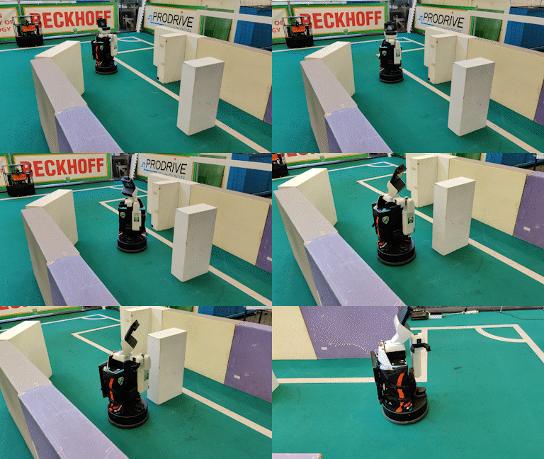
The GIF on the right side shows the result of implementing the algorithm on the robot. The algorithm works and the robot does find a path around the objects and through the corridor without collisions. However, the robot does show some abrupt changes. Upon calculating a new setpoint the robot abruptly stops and when this setpoint is found it abruptly starts moving again. This is off course not the neatest implementation. Another observation is that at a certain point the robot appears to have some trouble deciding where it's next setpoint is.
Some improvements we would like to introduce in the future is having the robot slow down gradually when finding a new setpoint. This would circumvent the abrupt motions. Another improvement would be to build in some hysteresis and updating the setpoint a bit less often. This should improve the decisiveness issues in the robot.
Exercise 4: Localization assignment 1
Assignment 1: Keep track of the location
The code for assignment 1 can be found on gitlab. This code prints the odometry data and the difference between the previous and the current odometry data.
Assignment 2: Observe the behaviour in simulation
By driving in a straight line forwards in simulation with the command: io.sendBaseReference(1, 0, 0); without uncertainty in the odometry sensor will result in a predictable increase in x position of the robot and no change in angle or y value of the odometry data. However in real life the data from a sensor always has a certain measurement uncertainty and the wheels can slip, leading to a different coordinate estimation based on the odometry compared to the actual position of the robot. In simulation the distance driven that is estimated by the odometry object. However, the laser scan data can also be used to estimate the distance that is driven. A block is placed in front of the robot and the difference in scan data between the previous and the current time step is added to a memory variable that stores the distance driven. This value can be compared to the one stored in the odometry object.
By driving straight forward without uncertainty in odometry data the following is observed in simulation:
- The angle and y-value in the odometry data is not changing and remains 0.
- The difference between the driven distance calculated with the scan data and that of the odometry data is quite accurately matching.
By driving straight forward with uncertainty in odometry data the following is observed in simulation:
- The angle and y-value in the odometry data is changing with small increments and thus does not remain constant.
- The difference between the driven distance calculated with the scan data and that of the odometry data is now bigger.
This proves that only relying on the odometry data for position can lead to uncertainty and errors in pose estimation. So it is recommended to use multiple sensors in the final challenge to make multiple estimations. By combining these estimations the uncertainty and error can be greatly reduced.
Assignment 3: Observe the behaviour in reality
The odometry data is calculated wrt a odometry frame which is different from the robot coordinate system, the global system and the laser scan system. During driving of the robot these frames come out of alignment. It was observed during experimenting that this disalignment indeed can be seen. As in simulation the coordinates in the odometry frame are compared to those inferred from the laser data. while driving straight forwards with the frames aligned it could be seen that both estimates are pretty close to each other, but after turning the robot the frames were no longer aligning. This resulted in a displacement in y-direction as well as the x-direction wrt the odometry frame. And thus both measurements no longer cohered.
Exercise 5: Localization assignment 2
Assignment 0: Explore the code base
- Difference ParticleFilter and ParticleFilterBase and relation
- Relation ParticleFilter and Particle classes
- Difference between propagation method of ParticleFilter en Particle
Assignment 1: Initialize the Particle Filter

The first constructor passes the world, weight and a generator pointer to the particle class, which then estimates a pose based on a uniform distribution, whereas the second constructor passes the world, mean, sigma, weight and a generator pointer to the particle class, which then estimates a pose based on a gaussian distribution using the mean and standard deviation.
In ParticleFilterBase a for loop is used to call the particle constructor and place the particle and its location in a vector called _particles for both constructors.
The particle constructor is finished by calling get_noise_sample_uniform() and get_noise_sample_gaussian() for x, y and theta and then using these estimated values to generate an estimated pose which is then initialised.
A screenshot of demo1 can be seen on the right side. This shows a gaussian distribution close to the robot, which seems to be correct. Assignment1 was run and passed all tests.

The Gaussian distribution uses prior knowledge to determine a better estimate. The uniform distribution estimates the probability for the robot to be anywhere on the map to be the same. The Gaussian distribution focuses mainly on your best guess, if it's incorrect it might spent a lot of resources on this area, whereas the uniform distribution spreads effort around the map equally.
Exercise 2: Calculate the filter prediction
The filter average returns the average of all the particle poses that are initialized. This does not resemble the robot position accurately, as it currently is exactly the middle of the map. The particles are initialized over the whole x and y of the map as well as over the [-pi, pi] and the average of this is the exactly the center of the map with a heading of 0 (which is north). The filter average might be inadequate when there is a big open space as the particles will be spread out far. This will result in a bad "resolution" in the particle filter and subsequently errors in estimations. Alternatively, if the robot has a limited amount of samples which it can use in the particle filter, it will suffer from the same resolution issues. This will also result in inadequate position estimations.
A screenshot of demo2 can be seen on the right.
Exercise 3: Propagation of Particles
Exercise 4: Computation of the likelihood of a Particle
- The Gaussian model is used to correct the range with local measurement noise
- The exponential model will compensate for unexpected objects
- The point-mass distribution will correct for failures
- The uniform distribution will correct for unexplainable random measurements
Normalization is now necessary because the likelihood otherwise might end up larger than 1