Mobile Robot Control 2023 Group 1
Group members:
| Name | student ID |
|---|---|
| Lars Blommers | 1455893 |
| Joris Bongers | 1446193 |
| Erick Hoogstrate | 1455176 |
Introduction to mobile robot control
On the robot-laptop open rviz. Observe the laser data. How much noise is there on the laser? What objects can be seen by the laser? Which objects cannot? How do your own legs look like to the robot.
- When looking at rviz quite some noise can be seen. Almost all objects in the room will be seen by the laser as it has quite a large range. Objects that the laser can not detect are for example black objects, as they do not reflect the light as good as other coloured object do, and glass objects as these refract the light instead of reflecting it. Legs of a person will also be detected by the robot. Legs to the robot look kinda like a "half moon shape" as the laser only sees the legs from one side.
Take your example of dont crash and test it on the robot. Does it work like in simulation?
- The robot works as in the simulation. The source file can be found in the folder "excercises-group-01/exercise1/src/dont_crash.cpp" on the groups Gitlab repository.
Take a video of the working robot and post it on your wiki.
- The video of the robot running the "dont crash" program can be found via the following link: https://bit.ly/3OOlmAF
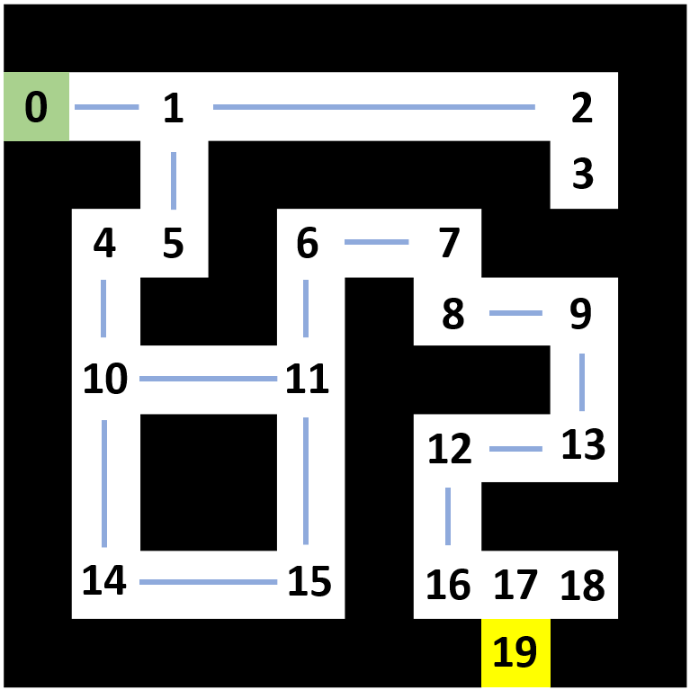
How could finding the shortest path through the maze using the A* algorithm be made more efficient by placing the nodes differently? Sketch the small maze with the proposed nodes and the connections between them. Why would this be more efficient?
- Finding the shortest path through the maze using the A* algorithm can be made more efficient by using less nodes as shown in the Figure below. All nodes that are not placed on an intersection (a node that is connected to more than two nodes) are removed from the maze as this does not influence the principle of the A* algorithm. The removal of these nodes has a positive effect on the computation time of the shortest path through the maze.

- Description of the approach: There will be repulsion effect on objects, which will result that the robot will avoid obstacles such as the bin. However, it does not yet work for walls which are located straight before the robot.
- Video simulation:
- Video real life: https://tuenl-my.sharepoint.com/:v:/r/personal/j_bongers_student_tue_nl/Documents/Navigation2video.mp4?csf=1&web=1&e=vi6A9W
Localization 1
Assignment 1:
A C++ program that reports:
- The information in the odometry message that is received in the current time step
- The difference between the previously received odometry message and the current message
Can be found on the groups gitlab repository in the folder "localisation_1/src/local_1.cpp". The program receives the sensor data from the robot and displays it in the terminal window.
Assignment 2:
In order to asses the accuracy of the odometry data received from the robot, an experiment is performed in the simulation environment. The robot is given the task to drive in a straight line parallel to the x-axis. The expected result would be to only see a change in x-coordinate and a constant value for the y-coordinate and rotation a. When performing this experiment in the simulation environment, the reported values of the odometry data of the robot indeed verify the aforementioned hypothesis.
When enabling the uncertain_odom option, the reported odometry data shows some clear sensor drift compared to the previous situation. Regarding the situation described above, the odometry data now also shows a change in y-coordinate which should not be the case as the robot moves parallel to the x-axis.
All testing performed in the simulation evironment should have the uncertain_odom option enabled as this setting will resemble the way in which the odometry data is received on the real-life robot. This setting needs to be turned on as the simulation environment acts as a "perfect" environment without any wheelslip and/or sensor drift. In real life these two factors do play a role and will cause some errors in the perceived odometry data. This problem can be solved by using a Recursive State-Estimation to get a better estimate of the location and orientation of the robot. This method uses an estimate of the location and orientation of the robot together with odometry and laser data to compute an estimate of the next location and orientation of the robot.
Assignment 3:
The difference between the simulation and reality is that the odometry data in reality shows the expected sensor drift and wheel slip while in the "perfect" simulation these factors are not present. The simulation environment with the uncertain_odom option enbaled resembles the situation in reality. The answers of assignment 2 have not changed after conducting the experiment.