Measurement plan and experiments
Back to the main page: PRE2015_3_Groep4
Measurement plan
Research question
Is it possible to know in what sleep phase a person is by analyzing the sounds that he/she makes while breathing?
Sub-questions
• What is the best way to measure the sound present in the bedroom?
1) High-frequency recording of the sleep measuring the pitch
2) Low-frequency recording of the sleep measuring the decibel level
• What conclusions can be drawn from the results we encounter?
What has to be done?
• Measuring
1) Measure the sounds of multiple persons their bedroom throughout the night.
2) Measuring multiple nights.
3 ) Measuring on a high-frequency sound level as well as on a low-frequency sound level.
• Processing the measuring results
1) Analyzing which method brought us the best results.
2) Determining if it is possible to use the data that we have for future work.
What are we going to use for the measuring?
For the measuring of the sound levels, an Arduino is used. This Arduino will be connected to a sound detector. We chose an Arduino Mega with a SparkFun Sound Detector. The results will be stored to be reviewed afterwards.
How are we going to evaluate the gathered data from the measurements?
We will use different methods to measure the sleep phase. The first one is of course with the aid of the Arduino. But we will control this measurement with an already existing application, which also measured the sleep phases during a whole night.
When and where do we do the measuring?
The testing will be done as soon as all the components arrived. The plan is to do as many tests as possible in about one week. Two persons will do the testing at their own home. This way there are twice as much testing results in the same time period.
The sound detector was recommended to us by Ruud van den Bogaert. It is more that suited for our needs, for it has both analogue frequency output and volume level or ‘envelope’ output. It also has a digital output that’s high when the volume rises above a certain threshold, which we won’t use.
low frequent or high frequent
Out of experiments can be concluded that the best way to measure the sleep phases was by sampling (relatively) low frequent. Namely, the data-logger was unable to log more than 1000 strings per second, which isn't enough for sampling high frequent. The Nyquist-Shannon sampling theorem[1] said, that the sampling frequency must be at least twice the highest component of the voice frequency via appropriate filtering prior to sampling at discrete times (4kHz) for effective reconstruction of the voice signal. So this theorem suggests that we need a sampling frequency of 8 kHz. We've to mention that we didn't expect such high frequent voices during your sleep, but it can be concluded that sampling with 1 kHz is much too low. And out of experiments could be concluded low frequent sampling gave sufficient results. (see the justification of the sleep graph below) So we've chosen this way of sampling.
data gathering for further processing in Matlab
We've used an Arduino and sound sensor to measure that sound during the sleep. These measured data is logged real time to a computer. To do this we first wrote a program which will print time, audio and envelope as fast as possible. These outputs will be logged on the computer during the sleep. The time will be in microseconds anywhere between 0 and 2^32, which is about 71 minutes. The audio is a 10-bit value (between 0 and 1023), which will typically be around 510. The envelope is also a 10-bit value which represents the amplitude of the sound. Because the amplitude is very low, this value is typically around 12. See code for the Arduino code.
Data pre-processing
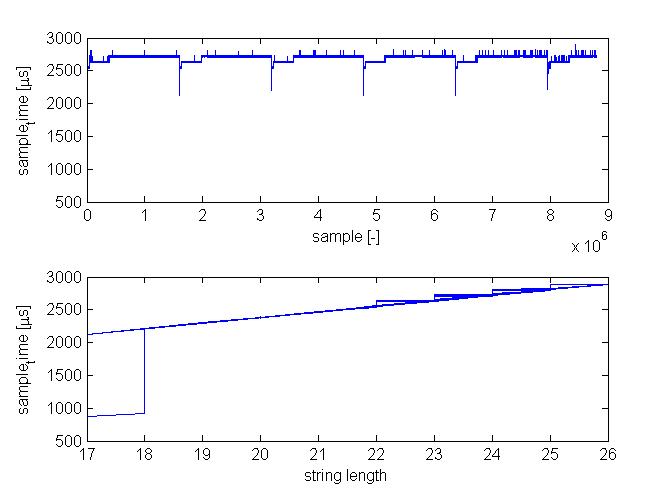
During a night, almost ten million lines of data are logged. These data can be analyzed in Matlab. Matlab will first 'repair' the time. Because 71 minutes is the highest value the Arduino can print, the time will overflow several times during one night. This has to be fixed by adding 2^32 µs to the time after the value drops. After that, some figures are plotted to verify the logging process. In the final script, this will not be done, but we need this to see whether the data is correct and usable in the beginning stage. For example raw input against time and the sample time for each sample, to find discrepancies the sampling frequency. In early versions, sample time against serial string length was also plotted, because this has a significant impact on sample time. This figure shows that the sample time increases with string length. A high variating sample time will influence the precision of the measurements. So we'll use a script which gives the output in a constant string length. Because of this, the sample time will be much more constant.
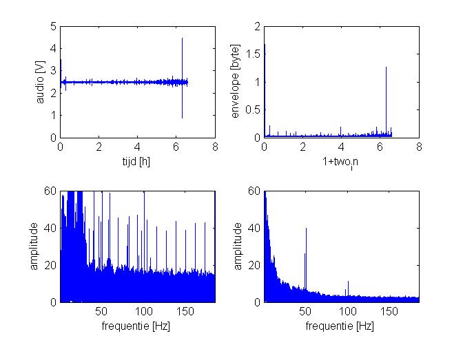
Below are some plots of the audio and envelope against time, and the amplitude of both against the frequency.
Removing bad samples
The mean sample time should be around 2000 microseconds. But this isn't always the case. Sometimes, the will be a print error. This can have a lot of different reasons, so it isn't completely preventable. These bad samples can't be processed in the next stages of the script, so it's necessary to remove these bad samples. The bad samples can be found by analysing the sample time. If the sample time is bigger than two times the mean sample time, it's a bad sample. By removing the bad samples, you've to pay attention that the next line of code will be connected with the previous one. So in most cases, it's necessary to remove more than one sample. For every print error, around the 32 lines will typically be removed. (maximum time is around 64000 microseconds. So this means if the sample time is around 2000 microseconds, that the number of samples is around 32.) So there will be removed for 0.06 seconds of data, which is neglectable.
A number of print errors aren't that much. Out of analysing the original data files it can be concluded that there are in almost all cases no more than 5 print errors. This amount doesn't influence the sleep graph visually.
Data processing
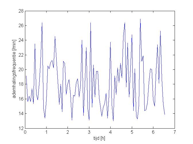
If the data is acceptable, it will be used to make a graph of the frequency of the respiration. The envelope signal is used. The data is divided into chunks of 4 minutes, these will be called frames. After that, a fourier transform is executed on each frame to get a graph of the frequencies and their amplitudes. Out of this graph, only the frequencies between 13/min and 27/min will be considered. This is done because the frequency of the respiration is between these limits. Out of the remaining frequencies, the frequency with the highest amplitude will be determined for every frame and used as the frequency of respiration for that frame. Now, we can plot the frequency of the respiration throughout the night.
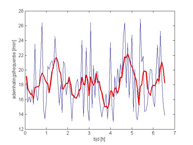
The data is taken from a real measurement (10-3-2016)
It doesn't seem to have a clear pattern. But when you plot a sliding average of the last five frames (thick red line), a more clear pattern will appear. This pattern cannot be verified for this specific night because it was measured without an already existing app.
This plot is from a single night. To get such a plot of every night, we have to measure more nights and try whether this algorithm also works for other nights (calibration-process). See the appendix below for the Matlab-scripts.
Determining moment of waking up
See the page code for a description of the algorithm.
Justification of our algorithm
We will check if the measured sleep cycle-graph is right. We will check this by measuring the sleep phase on two several methods at the same time. Of course, one method will be using our own algorithm. The second method will be with an application on our smartphone. The application is named SleepCycle. (see literature for more information about the App and how they measure the sleep phase)
"justification of the sleep phase
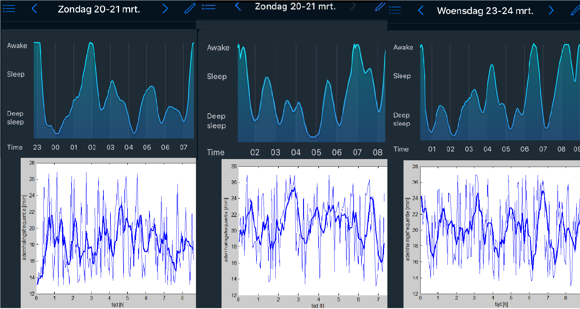
In the figure below are shown the results of three nights. The left and middle nights are measured on Sunday night the 20th of march by respectively Jeroen Ermers and Wesley van de Broek. The right night is measured on Wednesday the 23 of march.
Remark: All shown results in the figure above have the same variables. These variables are: frame length of four minutes, the blue line is an average of the last 5 points, a minimal frequency of 13/60 Hz and a maximal frequency of 27/60 Hz. These variables are determined out of the calibration stage. (trail and error by comparing the both graphs)
In general, our own algorithm shows much more tops as the application. But in most cases, if there's a peak on the graph of the application, there's also a top in our own algorithm. Some of the 'extra peaks' in our algorithm can be explained by the sub-peak in the graph of the application. For example, on the left night between 00:00 and 02:00, the line exist out of tree stages. The line isn't a smooth climbing line but stops climbing for two times. On these times, there are peaks in the graph of our algorithm.
The different heights of the peaks in the application aren't the same as in our own measurements in most cases. In our own measurements are the peaks mostly on the same height, while the tops in the application are variating a lot.
Another remark is the little delay in the thick blue line. The thick blue line is namely an average of the last 5 frames. This lead to a little delay, because the level of the thick blue line is also based on the data measured a few minutes ago. But in our imagination, the thick blue line is necessary to determine the best wake-up moment. It is namely necessary to plot an average line of the raw data. And when you're processing the data real-time, it isn't possible to look forward, so the only possibility is to look to the points a few minutes ago to make an average line.
Justification of the moment of waking up
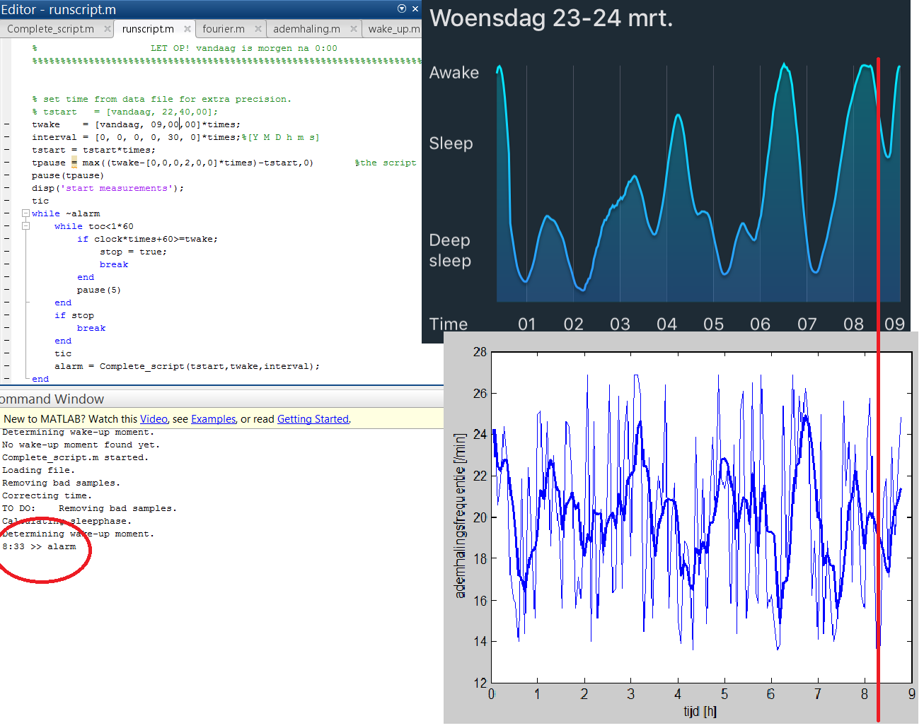
We've tested the whole script for many nights. This means that we have measured with our own algorithm, which will also determine the moment of waking up. The first night, we've only let Matlab print 'xx:xx >> alarm', where xx:xx is the best moment of wake someone. So Matlab won't play the music or put the lights on. We've done this, to see if it is really a good moment. This is easier to analyse when the person will sleep a little bit longer. The measurements won't be influenced because of the person is awake. The figure below is again Wednesday night the 23rd of march from Jeroen Ermers.
As shown in the figure above, the algorithm would wake Jeroen at 8:33. This is 27 before his outer-and-outer wake-up time. (shown in the script above as variable 'twake') The algorithm wants to wake Jeroen in the beginning of the wake-up interval. (show in the script above as variable 'interval'). The red line in the sleep phases shows the time the algorithm wants to wake up Jeroen. This moment of the sleep phase (around second nREM-stage) is in our mind the optimal wake-up moment.
conclusion
It can be concluded that it is possible to measure the sleepphase, so a sleep graph, during a complete night by sampling low frequent. By comparing the measured sleep graphs with the sleep graphs from the application it can be concluded that the graphs roughly show the correct the sleep cycle. But the height of the peaks isn't completely right. The question is, whether we really need the exact height of a top. Probably it's enough to know the positions of the peaks, and therefore the REM sleep, to determine the exact moment of waking up. So we realize that our algorithm doesn't describe the sleep phase perfectly, but the algorithm describes the sleepphase good enough to determine the best moment of waking up. Also, the determination of the wake-up moment is accurate enough. From another test, it can be concluded that the wake-up moment will be determined correctly. The algorithm wants to wake up the user just after the REM-sleep, which we see as the ideal moment waking moment.
