Embedded Motion Control 2019 Group 4
This is the CSTWiki page for group 4 of Embedded Motion Control 2019. The course Embedded Motion Control is about the design and implementation of software into autonomous robots. Application of the acquired knowledge is done to real-life robotics tasks and tested with robot PICO.
Additional recommendations that were pointed out during the lectures are:
- Perceive the world from the point of view of the robot
- Semantic knowledge of the environment is essential
- Incorporate what information is needed at which moment and how often it should be updated, with an eye out for computational power.
The statement above of the needed information at which moment is the main focus of our project. For example, planning is not important if you already know where you have to go and if you are not moving you do not have to avoid walls.
Because of this, PICO is chosen as the center of the universe and the map is changed to fit the location of PICO, instead of fixing a map point. Hence, PICO is the center of reasoning of all parts of the program. This year’s challenge is to move through a Hospital in order to visit a number of cabinets. The approach and solutions that are found are explained in the sections below.
Group members
| Marcel Bosselaar | 0906127 |
| Ruben Sommer | 0910856 |
| Jeroen Setz | 0843356 |
| Bram Grolleman | 0757428 |
| Martijn Tibboel | 0909136 |
Deliverables
Escape Room
The following ideas are used for the execution of the Escape room.
Escape Room - Plan
For the escaperoom challenge a specific strategy is determined. After initialization, PICO starts rotating and simultaneously scanning the room to find the door. In case no door is found after a full rotation, PICO determines the far-most corner and moves in this direction with half the distance measured. After this, PICO repeats this sequence. In case a door is found, PICO moves to a position 50cm in front of the door and faces the exit. A second scan verifies the location of PICO with respect to the door and corrects its position if necessary. After this, the end of the hallway is determined and PICO moves towards this point. After the goal is reached, PICO says it has reached its goal and shuts down. A schematic representation of the strategy is given below.
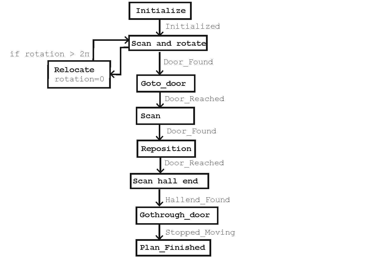
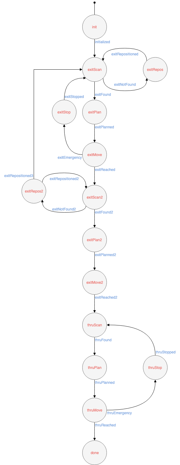
Out of the plan a finite state machine is introduced in order to maintain control over what is happening at all times.
Escape Room - Exit recognition
Before PICO starts looking for a door, the LRF data is first preprocessed into walls by a split and merge algorithm. Using these walls and the angle they have relative to each other, corners are found. Then, by looking at the different types of corners present in PICO's view, the location of any visible door is determined.
Split and merge method
The split and merge algorithm takes care of detecting walls in the LRF data. A wall is defined as a starting and an end point, a length and an index.
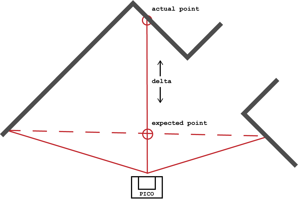
First, for every measured point the location in cartesian coordinates is calculated, using PICO as the center point. After this, PICO takes the leftmost and rightmost LRF-measurements and formulates the hypothesis that they are two points on a single wall. Then, the two points are used to calculate the expected middle point. Consequently, this point is compared to the real LRF-data measurement in the middle of the two points. Two checks are executed to verify the wall:
- The absolute distance between the expected point and real point is sufficiently small
- The length of the wall does not exceed the size of a door, to ensure no doors are overlooked
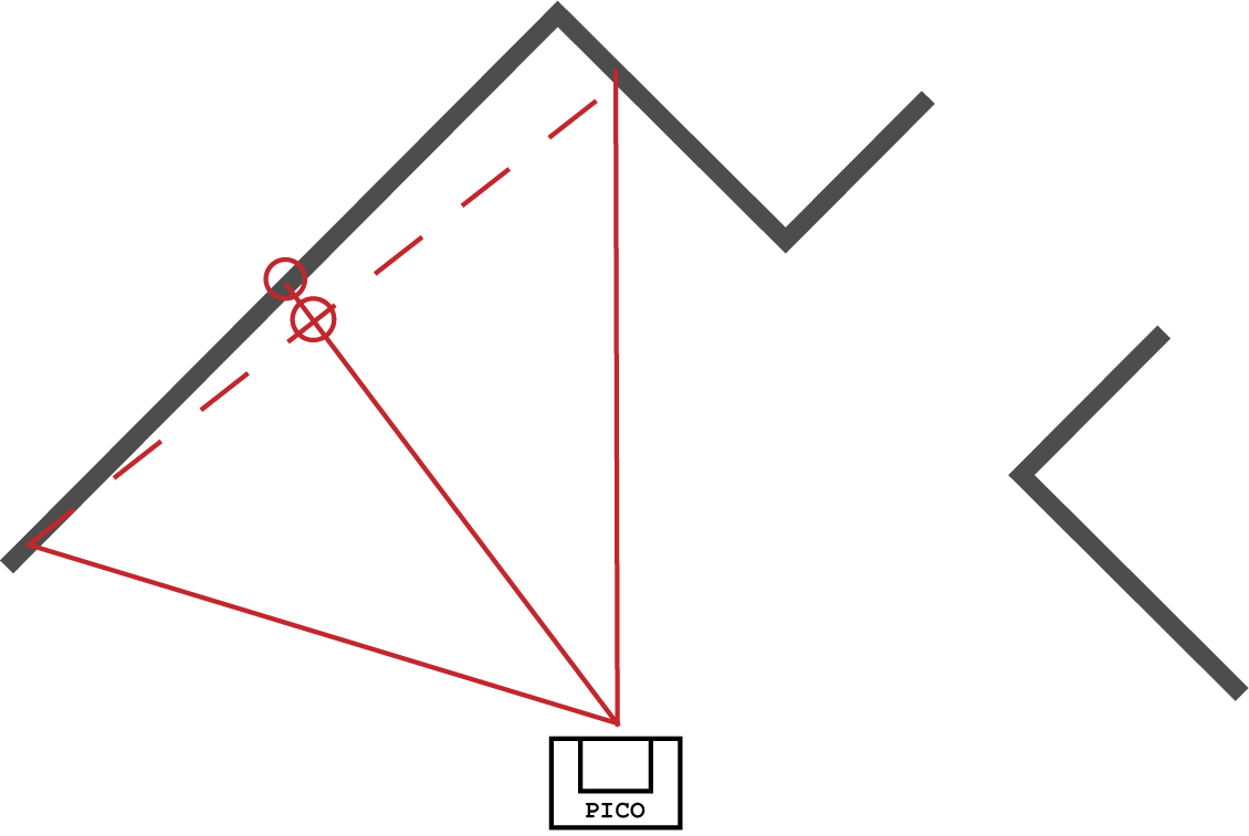
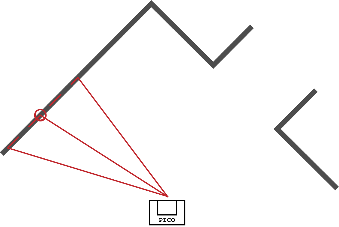
On a double succes the wall is confirmed. On a fail the wall is split into two separate walls on this middle point (the split). The process is then repeated on these two walls until all points are subdivided into walls, or splitting is no longer possible because a wall consists of only two points. Remaining is a large number of small wall sections that make up a room.
This is the point where the merge part of the split and merge algorithm comes in. When wall segments share an endpoint and the relative angle between them is sufficiently small, the walls are taken to be part of the same entity, and are merged into one larger wall. This way, the number of walls is reduced until the room PICO has perceived consists of a small number of straight walls, similar to how humans would perceive it.
The split and merge algorithm has proven to be very effective and has continued to be the base of the perception software in the Hospital challenge.
-
First step: Expected point is far away from real LRF-point; splitting wall.
-
Second step: Expected point is closer to the real LRF-point, but not sufficiently close; splitting again.
-
Third step: Expected point coincides with the real LRF-point and the two points are sufficiently close; wall found.
Corner recognition
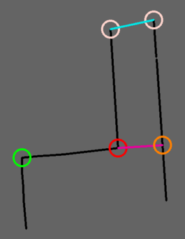
In corner recognition as used in the escaperoom competition, three types of corners are distinguished: Inside (90 degrees), outside (270 degrees) and endpoint corners. The first two are defined as a shared endpoint of two walls, where the walls have a certain angle respectively to each other. An endpoint corner is defined as the end of a wall at which no other wall is detected (i.e. a jump in LRF-data is measured at the end of a wall). In addition, so-called "flat" corners are defined, which can be seen as the spot on a wall opposite an outside corner, signifying the start of a hallway.
This method of corner detection has proven to be very effective and has played a major role throughout the project. The different corner types are shown in the image below. These are inside corner, outside corner, virtual "flat" corner and endpoint corners.
Door detection
By clearly distinguishing types of corners, doors can be found by looking at specific combinations of corner types. Three types of doors are possible:
- Door at the middle of a wall
- Door in a corner
- Door at end of hallway
Depending on the point of view, these doors consist of different combinations of corner-types. For instance, the door at the middle of a wall can consist of two corners of type "outside" or one "outside" corner and one "endpoint" corner.
To verify that a perceived door is actually a door, two checks were added. The first check is whether the width of the door lies within the expected margins, and the second check looks at the relative angle with respect to adjacent walls.
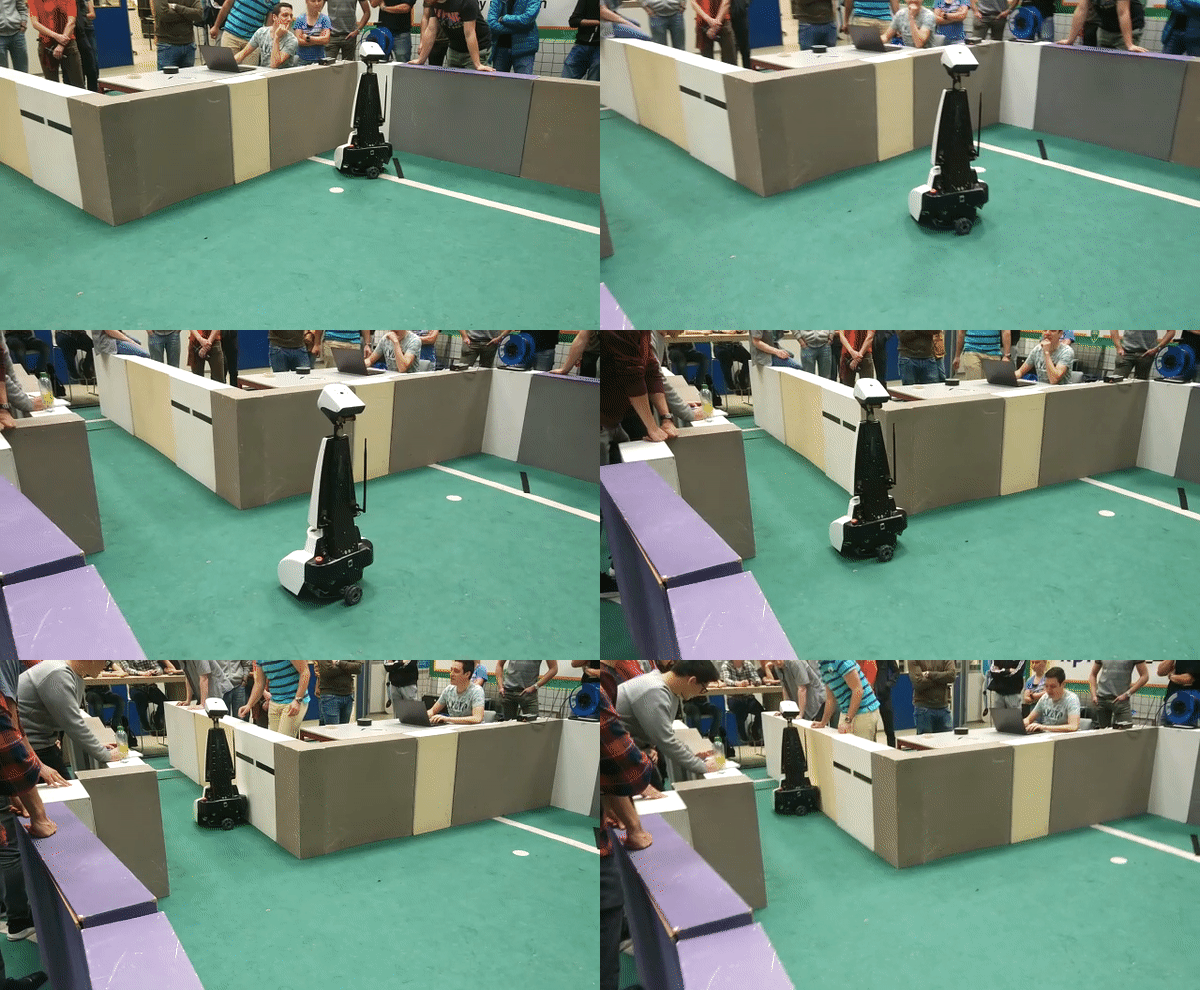
In the above figure it is already seen that a door in a corner is found and a door at the end of a hallway is found, shown by the pink and blue lines, respectively. Below an example is given where the door is in the middle of a wall and that is is recognised while rotating PICO

Escape Room - Testing
In real life PICO behaves different than in the simulations. A couple of things needed testing in order to stay on track of the global planning of the project. The main goal of every test date is given together with its result in the end.
PICO Test 1 (2019-05-08)
Goal: Have PICO detect the exit, and perform simple motion towards it.
Result: PICO moves in the correct direction, but the signal to the motors seems to be too low. Suspected problem: smooth acceleration, which is implemented to prevent slip and shocky movement, should be less smooth.
PICO Test 2 (2019-05-13)
Goal: Test improved smooth acceleration profile. Also test some parameter tweaks such as the emergency distance.
Result: Changed smooth acceleration profile helps a bit, but PICO still does not move to the desired location (moves less than expected). Suspected problem: PICO does not move by using odometry data. This should be implemented before the escaperoom challenge. UPDATE: movement on odometry data could not be implemented before the challenge day, because of the time. Therefore, a final check is implemented when PICO thinks it is in front of the door. Essentially, this contains an additional scan to find a door and a movements towards the desired location in front of the door.
PICO Test 3 (2019-05-16)
Goal: Test improvements done based on competition results. If available, test ideas that were previously generated but would only be useful for the final competition.
Result: Odometry still needs small tweaks, but the emergency stop works fine now. We don't take into account that there is an offset in the odometry frame, so a reset in this is needed.
Escape Room - Competition
In the escape room competition, we were potentially the team that had the highest high and the lowest low.
The designed algorithm worked perfectly and very quick. The door was found as soon as it came into view, and PICO decided to move toward the correct location in front of the door. The door was then immediately found again, and PICO's position in front of the door was made more accurate. Then, the exit of the hallway was detected immediately, and PICO drove towards its end goal.
However, due to the fact that odometry had not been implemented, the distances traveled were around 30% too short, meaning PICO stopped well before the detected end of the exit hallway. In addition, telling PICO to drive straight didn't actually make it drive straight, making it graze the wall.
The first improvement that needed to be done is the usage of odometry, as we're confident PICO would have exited the room within 30 seconds if it actually was were it thought it was. Secondly, the laser data should be used more frequently, updating plans during movement to keep things moving in the right direction. Improving the finite state machine to use fewer states and being more circular might also be a good addition.
After the challenge, an alternative FSM was thought of that reduces the number of states required and vastly improves accuracy. It is expected that the use of this state machine would have allowed PICO to complete the challenge correctly, even without the use of the odometry.

Hospital Challenge
The following section explains the different functions build and used in the hospital challenge.
Hospital Challenge - Software architecture
The figure below gives an overview of the elements present in our software, with some of the most important functions these elements run, the data present in them, and the data sent around between them.

The control over which function is allowed to use what data comes from the definition of the functions. Each function gets access to certain variables that are relevant for their functioning.
Standard access is read-only, so the function basically creates a local variable that can be accessed by elements within the function.
Data that should be altered, represented by the arrows returning into the world model, is fed into the function with write permissions.
Hospital Challenge - Finite state machine
Due to the hospital challenge requiring different functionality from the escape room challenge, a new finite state machine was developed, visible below.

Explanation
In this state machine, there is once again an initialization state, called init. Once PICO has been initialized, which is checked by grabbing LRF and odometry data and seeing whether it is correct, the event initialized occurs, and the state is set to initMap.
With the initialization of the state initMap, the localization flow has been started. This flow works by using the initMap state to have PICO gather LRF data, until such a time that the desired data has been collected. Once this happens, the initFit state is used to attempt to fit this data to the map, and orient the map correctly with regard to PICO. Should a fit prove impossible, the state initRepos will become active, in which PICO will attempt to reposition itself in a different location, and try to map and fit itself again.
Once PICO has localized itself, the state will switch to goalSelect, leaving PICO in the global movement flow. Here, PICO will select the cabinet it should travel to from the array created by user input in the goalSelect state. Once this has been done, the goalPlan state will use our rapidly-expanding random tree algorithm to generate a path to the selected cabinet.
The goalMove state handles the actual movement along the generated path to the cabinet, as well as dynamic obstacle avoidance. From this state, two escapes are possible. The first and most important is the goalAvoid state, triggered by the goalEmergency event. As the event implies, this state is designed for avoiding an emergency, and should only occur when an object suddenly comes too close to PICO, as the dynamic obstacle avoidance should keep PICO from reaching the emergency state during normal operation. The goalAvoid state then reorients PICO to a safe location, and the goalPlan state becomes active again.
Should PICO get stuck in the goalMove state and not be able to reach its target, the objectFound event is triggered, setting PICO to the goalObject state. In this state, PICO will add the unexpected object to the map, and once this is done the goalPlan state will become active again, and will plan a path around the new object that was added to the map.
The end of the global movement flow is signified when PICO has reached a point of half a meter in front of the cabinet. From this point forward, PICO will use its LRF sensor to enable precise local movement. The first state in this flow is cabFind, in which PICO will attempt to recognize a cabinet from its LRF data. Once this cabinet has been found, PICO will move towards it in the cabMove state, once again with an emergency avoid state.
When PICO has reached the desired position in front of the cabinet, the cabStop state will become active, in which PICO will pause in front of the cabinet and exclaim what is happening. Then, in preparation for movement to the next cabinet, the cabTurn state turns PICO around by 180 degrees, so he's looking away from the cabinet, and the global movement flow is once again initiated when the event cabTurned is thrown.
Global and local movement will keep occurring just as long as there are more cabinets in the array of supplied cabinets, when the event goalReached occurs. This event leads to the done state, signalling PICO to say goodbye and terminate the program.
Implementation
The state machine as described above has been implemented in the software as an enum type variable for the events and for the states. This type of variable can only have the values of the states/events, declared in its generation.
The monitor function is the only function that can alter the states, and it will do so based on the events generated by the other functions. For instance, when the event goalSelected is thrown, by way of the variable E having value goalSelected, the monitor will change the state to goalPlan, by way of changing variable FSM to goalPlan.
The perception, planning, and control functions will then display different behavior depending on what the value of FSM is. This is achieved by creating multiple successive if-loops that describe the behavior in a certain state or states.
Conclusion
With the finite state machine as described above, we have developed a usable way of controlling PICO's discrete behavior. Due to multiple loops in the state flow we believe to have kept the states to a sufficiently low number, while still having very clear states for very clear behavior. The implementation is susceptible to errors, as the events are not coupled to the state PICO is currently in, but with the use of the figure no programming errors have occurred.
Hospital Challenge - Localization
For the hospital challenge it is crucial to be able to localize accurately. With the RRT relying on the location of PICO on the map, the idea is to update the localization every time the robot needs to make a new path. In between two setpoints of the path, the odometry is used to know the current location and this is assumed to be 'good enough'. If PICO may run into trouble of any kind, either the (dynamic) obstacle avoidance or the state machine compensates for this. In this case, the robot goes to a 're-planning' state, where it also updates the location again. In this way it is never a problem if the accuracy of the localization is a bit off. The procedure of elaborated below.
Point matching
PICO is localized as follows:
Before the final challenge, in order for PICO to localize, the corners of the map are given the type 'outside' and 'inside' by hand. When the program is started, a calculation is done over the map information. All corners are specified with the right corner type 'inside' or 'outside' corner, which is also done for the LRF data as explained in the escape room challenge. For all corners of the map is the distance between the point and all other points calculated for use in the future.
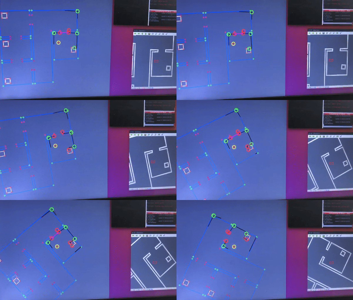
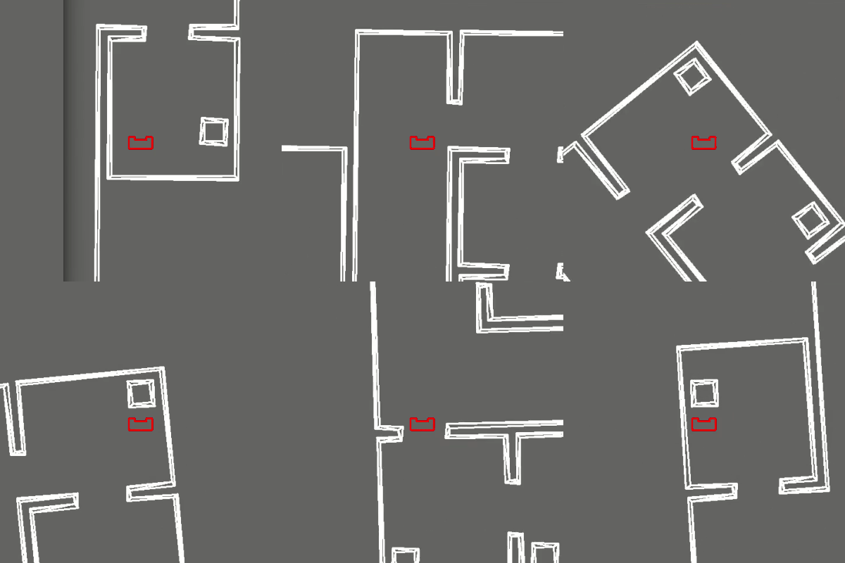
Within the localization script a loop is made through all corners of the map and all corners that are specified in the LRF data. A point of the LRF data is checked if it has the same kind of corner as the map point. If that is true, another point of both data sets is checked if this has the same kind. When this holds, a distance is calculated between the points of the LRF and then checked if this distance is near the distance that it should be compared to the map. (which is stored in the beginning) Summarizing, this means that a wall with 2 points of the LRF data is checked if it is suits to be fitted to a wall of the map. A visualisation of this is given in the following figure:

Next, this is done for another three walls, while aborting if one of the statements does not hold. This reduces the amount of possibilities of the best fit and the possible fits are stored in an array. After this, the script uses the stored fits to calculate a location of PICO in the map with the given distances from the LRF corners that are fitted in the fits. The different that come forward are analysed on the amount of occurances and unfeasible locations (outside the map for example) are removed from the possibilities.
From the locations that are found a mean location is calculated together with the guess (from the odometry data) where PICO possible could to obtain the final location of PICO. Accordingly to the location of PICO the map is translated and rotated in order to fit the map over the LRF data. This way the planning can be done easier, because it is assured that PICO is at the origin of the plot.
A problem occured while making this way of localizing. The localization had a lot of 'unwanted' locations, so that is why the above filters were added. This solved the problem, but still a offset remained within the localization. Later on it appeared to be a problem within the shifting of the map, because we were using multiple coordinate system which made reasoning pretty hard. In the beginning we thought it was the uncertainty of the found points that gave this offset, that is why we also looked at other localization options. Which in the end, turned out to have the same problem.
Alternatives
In an alternative localization procedure than described above, a door finding and cabinet finding algorithm can be used. This algorithm comes from the exit recognition that was used for the escaperoom challenge and worked very well. In the hospital challenge, doors are recognised in the same manner as the exit was detected in the escaperoom. Cabinets are defined as a set of corners with certain properties: corner distance and corner type. This way, the location of PICO can be determined by using the distances of the LRF corners. This alternative worked much faster than the other localization algorithm, as hardly any calculation is required. However, this option is heavily based on the geometry of the starting area, and is therefore not very generic.
Another alternative that is considered is the use of a particle filter for localization. This is a well known type of localization and some examples can be found online. The accuracy of a particle filter improves over time, because more samples are used. Particle filters are not used in the design, because it would be much of an 'overkill', since the starting area is known and the rooms have enough points of recognition (think of distances and corner kinds etc). Therefore it is chosen to localize with an in our opinion more elegant algorithm where less computational effort is required.
Hospital Challenge - Path planning
Path planning is defined here as finding a way from point A to B based on a known map while avoiding obstacles on this map. In general there are four different approaches to path planning for mobile robotics:
- Cell decomposition
- Divide the map into a grid and define obstacles as cells which can not be used for movement. Then an algorithm as A* or Dijkstra can be used to find the (optimal) path from A to B.
- Potential fields
- A map is converted to a potential field map in which obstacles have high values and free space low. This way a path from A to B can be created which follows the lowest potentials.
- Sampling based
- A sampling based algorithm finds points in the free space of a map and tries to connect them. Then a path is found from A to B following these points. Examples are a Rapidely-expanding Random Tree (RRT) or a probabilistic roadmap.
The requirement set for a path planning algorithm was to avoid a grid (to prevent scalability issues and limited cell resolution) and potential fields (as followed from the Do's and Don'ts lecture). Therefore one candidate remained: sampling based. The choice was made to use a RRT algorithm as is seemed easier to implement compared to a probabilistic roadmap. The benefit of using such a path planning algorithm is the genericity. It does not need any predefined points, cells or possible paths. It can find a path on any given map with obstacles.
Rapidly-expanding Random Tree algorithm
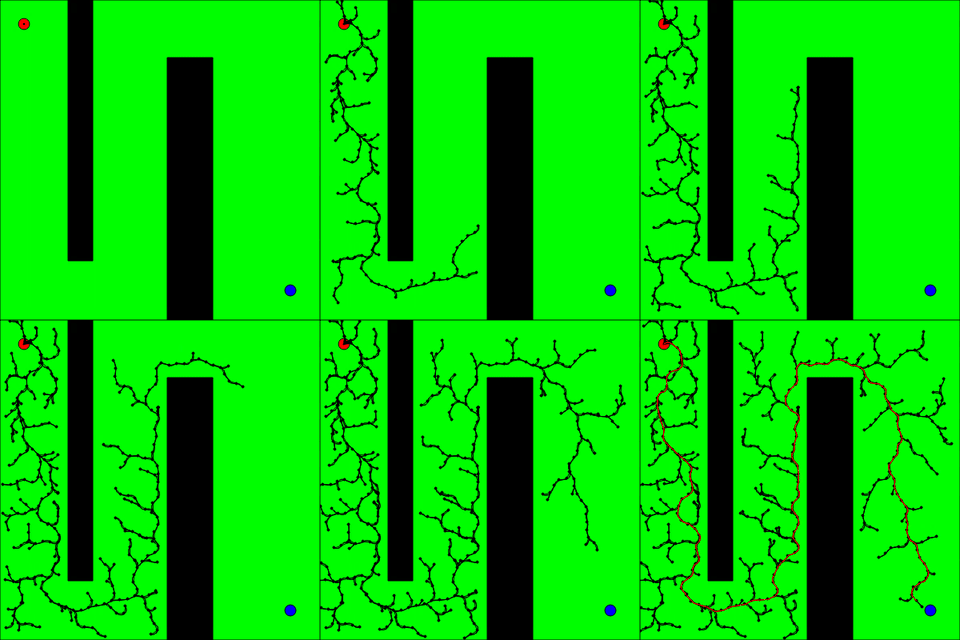
A RRT algorithm starts with a root node. In this case the initial position of PICO. In each iteration of the RRT-algorithm a random point is created in the space of the map. The closest node of the tree to the random point is chosen to extend the tree in the direction of the random point. The connection of the newly placed node will be checked for validity (i.e. not colliding with obstacles on the map). This way the random tree will eventually span the complete free space. The algorithm terminates if the goal point B is reached with the tree. An open-source existing algorithm is used which creates a basic random tree. This is modified to work with our software. Two (major) additions are done to the existing algorithm.
RRT end point bias
To ensure a quick convergence of the tree towards the end goal (point B), an endpoint bias is used. This means that every few iterations the algorithm does not use a random point is space but the end goal. This way the tree will be extended in the direction of the goal. This proved to achieve a much faster algorithm which required a lot less iterations to find a path. The end point bias may to be too large (i.e. take every other random point as the end point) as the algorithm can get trapped in corners between obstacles.
RRT path splitting
A drawback of the RRT algorithm is that it will find a path which is generally not optimal. To optimize the found path, a splitting algorithm is used similiar to the splitting algorithm used to find walls in LRF data. In the first step, the splitting algorithm tries to connect the start and end point of the path to see if they can be connected with a straight line without colliding with obstacles. If this fails, the check is done using the middle point of the path. This is done recursively to optimize the path. In the worst case scenario the original path will be retrieved again. The RRT splitting method showed to create nice straight lines between all points on the path, this still does not create an optimal path, but an optimized version of the original found path.
Resulting pathplanner
With the two improvements to the random tree path planner implemented, the final result is shown below. A path is created based on the obstacles (walls and cabinets) in the JSON file of the hospital challenge from initial position to cabinet 0. First a random path is found, in which the influence of the endpoint bias is clearly visible. Afterwards the path is approximated by straight lines using the path splitting algorithm. This results in points which can actually be followed smoothly by PICO. The path is shown not to cross any obstacles. Obstacle lines are slightly extended to prevent pico from driving too close to wall corners. This could be improved by blowing up obstacles instead of just extending them. When the path is created, it consists of an array of points. An extra orientation is added to these points in order to let PICO orient itself in the direction in which it will drive to the next point. (Note: The image visualization is not the actual speed of the pathplanning algorithm, this could be much faster or slower depending on the map.)

Hospital Challenge - Movement
The movement of PICO from a start position to a cabinet is divided into two parts: global and local movement. This is also reflected in the finite state machine. In global movement PICO follows the path created by the RRT path planner. This results in a path to a location which is 0.5m in front of the cabinet. Once this location has been reached, PICO switches to the local movement flow. This basically means it has to find the cabinet and drive to the required distance of approximately 20cm in front of the cabinet.
Hospital Challenge - Global movement
The global movement flow is visualized in the finite state machine diagram. It starts with selecting a goal (State = goalSelect), which is an entry of the list of cabinets that should be visited. A counter is used to keep track of the number of cabinets that are already visited. If all cabinets are already visited, the program is shut down. Once the goal is selected, a path is planned using the RRT pathplanner (State = goalPlan).
Once the global path is created, PICO has an array containing positions (x,y,theta) which define the path. The trajectory() function in the control section sets the velocities needed to reach the next point in the path. Once PICO is within a certain range of the target path position, the next point is selected to drive to (State = goalMove). This prevents PICO from stopping in between points and ensures he moves smoothly along the path. Once PICO is driving to the final point of the path, the required distance to the endpoint is much smaller to ensure PICO reaches his final position. During the goalMove state, two special situations can occur: Emergency or Stuck. The emergency state requires PICO to stop and plan its path again. The Stuck situation appears when PICO does not move significantly for a certain amount of time. This means PICO has probably encountered an obstacle in its path which was not on the map, or is trying to avoid an obstacle, which has driven him into a corner. PICO will then scan the room and add obstacles in sight to the map. Then the state is set to goalPlan again. The obstacles found in its path will be taken into account when planning a new path. When the final location is reached, PICO will switch to the local movement flow.
Hospital Challenge - Local movement
As stated in previous section, after PICO has reached its destination determined by the RRT, PICO switches to a local movement flow. In this flow, PICO moves towards the cabinet based on LRF-data. This is done in a few steps: First, PICO scans the room. In this step LRF-data is updated and the algorithm is started which finds walls, doors and corners, which results in an updated world model. Secondly, PICO searches for corners in the world model with certain requirements (distance to PICO, distance between corners and corners of type "outside") to find the front wall of the near cabinet. This step is also used to update the position on the map based on the LRF data and the cabinet PICO is looking at. If the cabinet is not found, PICO starts rotating and searches for cabinets again, until the cabinet is found. Thirdly, PICO moves to the desired position in front of the cabinet on odometry data.
Hospital Challenge - Obstacle avoidance
In order to have PICO move through the hospital safely and fast and yet prevent live- and deadlock situations, two layers of obstacle avoidance were implemented. The first layer, the dynamic obstacle avoidance, has as primary function to exert repeling forces on PICO pushing it away from obstacles while driving. The second layer, the static obstacle avoidance, becomes active when the chosen trajectory can no longer be followed, even with the help of the dynamic obstacle avoidance. Its primary function is to recognize these objects and add them to the map to enable the planning of a path around it.
Dynamic obstacle avoidance
The avoidance of obstacles during driving, and which does not require PICO to stop and plan a new route, has been labelled dynamic obstacle avoidance.
Two different algorithms were developed, with a similar thought behind them. The first was to look at the nearest point to PICO, and push PICO away from this point. The biggest issue with this method was that PICO will jitter immensely when moving through narrow hallways or similar features. In order to solve this, a second algorithm was developed. This second algorithm has a similar functionality, but it looks at all points that lie within a certain safety range, and pushes PICO away from them simultaneously. Different strengths of the repulsion are defined in x and y-directions, allowing finetuning of the avoidance behavior.
Implementation of the dynamic obstacle avoidance has been done as follows. First, the trajectory function determines the velocities required to move to the next point in the path, including initial acceleration and final deceleration. These velocities are entered into the avoid function, which uses the data from the LRF readings to push PICO away from any objects that are too close for comfort by altering the velocities that were input. Finally, the slow function slows PICO down when too close to objects, to ensure PICO can stop quickly when emergency situations might occur, and to scale the velocities down to the maximum when the avoid function has been too aggressive in its avoidance.
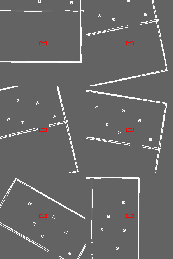
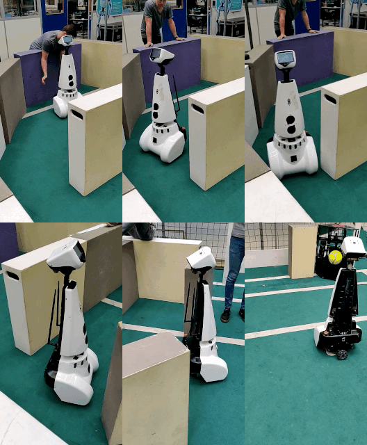
The image below on the left shows how the obstacle avoidance works in a simulation enviroment. PICO is only aware of the wall in front of him at the starting position and plans a path to a location 4 meters in front of him. He succesfully avoids all small obstacles in the adjoining room. The second image displays a test done on PICO. Again he is only aware of the first wall in front of him and succesfully avoids the obstacles on his path.
 |
 |
Static obstacle avoidance
The recognition of obstacles which cannot be avoided by repelling forces alone and do require PICO to stop and plan a new route, has been labelled static obstacle avoidance. Next to recognizing unexpected obstacles and adding them to the map, obstacles that have been added to the map and are no longer present in the environment should automatically be removed.
Detect new obstacles
A situation in which dynamic obstacle avoidance is no longer sufficient is communicated through the event objectFound setting the state to goalObject. The static obstacle avoidance then adds any found walls (lines) found in the LRF data to the map as if they were obstacles. E.g. a box of which two sides are visible will be defined as two separate obstacles.
Next, the obstacles that are defined multiple times (overlapping lines) are merged and obstacles that are recognized as being on the JSON map are removed. In this procedure, obstacles are interpreted as lines. The algorithm looks at the relative angle between lines, the perpendicular distance from one line to the other and checks whether the lines overlap. If all hold, a new obstacle is defined as a combination of these lines. The two initial obstacles are removed. The same checks are executed to filter any walls from the obstacles.
With the updated version of the map, the path planning is now able to re-plan the route towards its target, now taking into account the detected obstacles.
Detect missing obstacles
To have a robust system, not only should it have the possibility to add obstacles, but it should be able remove them when they are no longer present. As part of the static obstacle avoidance, the function removeObstacle takes care of this.
The function loops over all obstacles found previously and checks whether their corners should be within vision range and the view on the obstacle is not obstructed. This is done by checking if a line between the corner and PICO is crossed by a line of data from the LRF scan. If not the obstacles should be visible. As this function is used before adding new obstacles, an obstacle in sight which is still in place will be added to the map again.
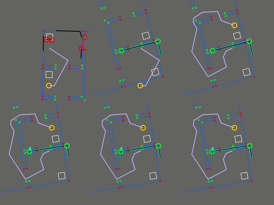
This way paths that were obstructed before will be accessible by the robot again when the obstacles as well as wrongly detected obstacles are removed. The image below shows an example of how PICO is able to plan around an obstacle found. In this case a door which seems to be open in the map, is actually closed. PICO made a path from cabinet 2 to 0. When following the path an obstacle (the closed door) is detected, added to the map and planned a new route. As the localization at this point was not fully correct, the obstacle is placed on the map with a slight offset.
Hospital Challenge - Testing
The following tests were planned and performed for hospital functionality.
PICO Test 4 (2019-05-29)
Goal: Setup of test area: two rooms, with matching .json and sim map (similar to items provided on Wiki).
- Main priority: Localization
- Plan to two cabinets, first far away, second back in start area, move to both
- Initialization to RRT planning.
- Dynamic obstacle avoidance
- Create a test case, just drive straight ahead and place an object in PICO's way
Result:
- Pico drives backwards due to no odometry reset
- Program crashes at wall merging (probably due to array size in recursive function)
- Turn all arrays into vectors so issues like this can never occur.
- Wall avoidance trough door is too tight. Keeps repositioning in door, does not drive trough.
- Program stops after emergency, does not plan again.
- Update FSM flow, create functionality for replanning.
- Pico plans a path trough walls because it drives on lrf data only
- Enable planning on JSON map.
PICO Test 5 (2019-06-03), PICO Test 6 (2019-06-05) and PICO Test 7 (2019-06-11)
These tests were mainly on testing a lot of small things and problems that occured while testing.
Goals:
- Test the localization algorithm and the dynamic obstacle avoidance.
- Robustness of localization algorithm
- Should work in any orientation, and should not determine incorrect location.
- Robustness of dynamic obstacle avoidance
- PICO should be able to move through doors without stopping or jittering.
- PICO should be able to move through hallways without stopping or jittering.
- PICO should be able to avoid moving objects.
- Functionality of static obstacle avoidance
- Recognize when an issue has occurred
- Plan a new path around the obstacle
Results:
- PICO sometimes drives backwards, even though this was supposed to have been solved.
- ODOM.reset() was not called after initialization, has been added to the software now.
- PICO does not yet plan using the JSON map, only on the LRF map.
- Enable this in RRT planning function.
- Bram’s avoidance algorithm works better right now, and we will continue working with this.
- Marcel’s algorithm requires at least too much tuning, and perhaps has more issues.
- PICO moves correctly through hallways.
- PICO moves correctly through doors.
- PICO sometimes hits walls directly ahead.
- Try finetuning the avoidance parameters in that direction.
- PICO returns to 0 after movements.
- Update map and reset odometry after movement.
- Update map accurately when in front of cabinet.
- It is unclear whether PICO always orients itself correctly in front of the cabinet.
- Atan2 definitions need to be checked, rotations might get flipped.
- Is the localization accurate enough?
- Tolerances present in both RRT path and in next point selection, might make PICO drive through walls.
- Visualization doesn’t work during movement.
- The room and location on map could be updated more frequently
- Orientation-dependent emergency might be interesting.
- PICO is wider than long.
- Localization in test does only work iff pico finds 4 corners. If more or less corners are found, translation matrix went to inf.
Hospital Challenge - Simulation
To show how the final program works, a full simulation is done on the competition hospital map. During this simulation PICO is told to visit cabinets 0, 1 and 3. The complete program is used as described above. Note that the GIF is played at 1.7x speed with 5 FPS due to the limited available file size. A full video of this simulation can be found in ZIP attached.
 |
 |
Hospital Challenge - Competition
The hospital challenge consisted of two trials. Within these two trials we had the chance to show our skills to a bigger audience and to the organization of the course. The localization problem was known but hopes were to show as much of our built functionality as possible.
The first trial was not a succes. The initial localization of PICO was to place itself outside the hospital map. Therefore the pathplanner could not find a path to the first required cabinet and PICO remained standing still on its starting position.
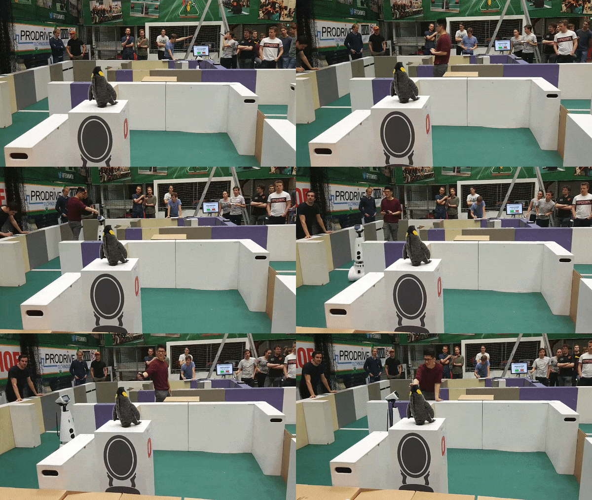
The second trial worked out a lot better. The initial localization was correct and PICO was able to plan a path to the first cabinet. When following the path PICO did not update the localization (continous localization was not finished) and therefore only relied on its odometry data. This proved to be too inaccurate to use in this hospital challenge. PICO stranded next to a door where he had to replan his route. Here PICO could not localize itself again correctly and therefore could not plan a new path to its destination.
Conclusion
The Embedded Motion Control course of 2019 proved to be a challenging assignment but was received with lots of enthusiasm. It is not often you get a chance to just play around with a robot like this. Besides the requirements set by the course, additional goals were set by ourselves as deducted from the lectures accompanying the course. These included semantic knowledge of the environment, selective use of information, a world view as perceived by the robot and to avoid using a grids.
Escape Room challenge
The first requirement was already fulfilled to a large extend by class definition of walls, corners, doors and later cabinets. The split and merge algorithm allowed the recognition of these semantic concepts in the LRF data in an accurate yet efficient manner. Rather than mapping out the entire area, the algorithm looked for a door and next for the end of hallway, fulfilling the second and third goal by only making use of information needed to fulfill the task at hand and defining the door and end of hallway positions as seen by the robot. The effectiveness of these concepts was clearly visible during the escape room challenge as the door was found immediately as it entered PICO’s field of view. The task of the driving towards known target however was underestimated and PICO was unable to reach the exit.
Hospital challenge
For the hospital challenge, driving on odometry was successfully implemented and reinforced with a powerful ‘dynamic obstacle avoidance’. Speeds were adjusted when getting close to obstacles while adding repelling forces to PICO from any obstacles around it.
The fourth goal mainly played a role when coming up with a path planning algorithm. The solution for grid-less path planning was found in a RRT algorithm, which was extended with a small bias to make it converge faster and our own split and merge algorithm to generate a smoother trajectory. The addition of static object detection and updating provided the option to find alternative routes in case the way was blocked, forming a strong combination with the path planning algorithm. The whole system was controlled by a strong and extensive finite state machine. Yet through the smart use of loops it remained relatively compact while at the same time adding to its robustness.
The only weak point in the system was the localization, which was neither strong enough to always determine its location regardless of its position, nor had the ability to use priory acquired knowledge to update it. The localization was built keeping in mind the use of semantic concepts and to make PICO the center of the world, but this proved to be too hard for the time given. This caused us to fail the final competition.
Due to the lack of proper localization, the competition has not shown the full potential of the result of this project. Yet we are convinced that there are some very powerful tools among the created software of which we would be happy to see them reappear in the upcoming years. Hence, in the end group 4 is happy with the progress that was made within the project. We thank the organization of this course for this opportunity and help with the assignment.
Recommendations
The implementation of localization was unsuccessful in the project. The use of semantic concepts as recognizable features however had lots of potential, given more time to implement it. The algorithm would fail however when multiple rooms show the same features, in which case it could be combined with the option to have multiple hypothesis on its current location. Yet many good alternatives present themselves.
Also a lot of wasted hours were spend on the endless conversion of coordinates from PICO’s view to the map and back, because they worked in different coordinate systems. Our recommendation would be to from the start convert these to work in the same system. This will not only save on computation time, but will mainly help understanding the systems and reduce the chance on errors.
Code
The following snippets give a good representation of how the software for this project was structured, and how it did what it was supposed to do.
- Overall functionality
- State changes
- Effect of state on functions
- Methods in classes
- Dynamic obstacle avoidance
- Velocity planning
- Complex classes
- Functions within functions
- Splitting of the RRT path
Minutes
- Meeting 1 (2019-04-29)
- Meeting 2 (2019-05-06)
- Meeting 3 (2019-05-08)
- Meeting 4 (2019-05-13)
- Meeting 5 (2019-05-20)
- Meeting 6 (2019-05-27)
- Meeting 7 (2019-05-29)
- Meeting 8 (2019-06-03)
- Meeting 9 (2019-06-05)
- Meeting 10 (2019-06-12)
- Meeting 11 (2019-06-20)
