Embedded Motion Control 2015 Group 3/Localisation
Localisation
This page is part of the EMC03 CST-wiki.
This page goes into details about localisation.
Requirements of Localisation
In order to be able to locate itself within its environment, the robot needs information. The is required to obtain global position data:
- global x-position [m]
- global y-position [m]
- global a-angle [rad.]
The error in the position data must be quantified and must be minimized, in order not to make mistakes in the location in the long run. For example, if the robots x-and y-coordinates differ due to an error, the robot will think is it at a different location, whereas it actually is standing still in exactly the same location and position.
The sensor data required to obtain the above mentioned position data are the following:
- odometry: global x [m] , global y [m] , global a [rad.]
- LRF: all laser ranges [m]
- velocity input to robot
Method of localisation
The robot will need global coordinates. There are two sensors which it can use to determine these coordinates. However both sensors have their own drawbacks.
- The odometry sensor provides global x-y coordinates and angle. There is not much variance in the data of the sensor, but there is a drift (bias) that will accumulate over time. The odometry data can be viewed as feedforward information for the system.
- The LRF sensor provides 1000 ranges [m] with distances to objects over a scope of 270 degreess around the robot. This sensor shows no bias, but has a variance however. Furthermore the LRF data does not provide the global coordinates that we want with its raw data. Therefore these ranges data have to be converted into additions to the global coordinates. The LRF data can be seen as the Feedback loop of the system.
When the robot starts its program initially, the global coordinates will be all zero. So the start position of the robot determines the direction of the x- and y-axes. The data from the odometry and the LRF will be updated at each time instant. The odometry just works very intuitively: it tells you how far you have moved based on wheel-rotation. In the case of LRF however, the following happens: It measures the distances to the objects in the environment at time t0. It measures again at t1. The difference in distance, converted to the wanted coordinates, should be equal to the odometry data. Of course this will not happen due to the errors in the sensors, but that is why a filter is used to filter the data in between each next update step.
A Kalman filter is used to filter the data obtained from odometry as well as from LRF, in order to maximize the accuracy.
Kalman filter
The kalman filter uses an update cycle with two steps. In the first step the new position is estimated based on the previous position and the input. An estimate of its error is then made which is used in the second step. In the second step data from measurements is used to correct the estimated position. Since the definition of the directions of the x and y axis is arbitrary, they are aligned to the corridor in which pico starts. The algorithm that is used is shown in the figure below:

The various variables used in the figure above, are explained here:
[math]\displaystyle{ \hat{x}_k^- }[/math] is the predicted ahead state variable at discrete time instance [math]\displaystyle{ k }[/math]. This column vector consists of the global x-position, global y-position and the global angle. So logically, [math]\displaystyle{ \hat{x}_{k-1}^- }[/math] is the same vector at a previous time instance.
[math]\displaystyle{ A }[/math] is an n by l matrix that relates the state at the previous time step [math]\displaystyle{ k-1 }[/math] to the state at the current step [math]\displaystyle{ k }[/math], in the absence of either a driving function or process noise.
[math]\displaystyle{ B }[/math] is an n by n matrix that relates the optional control input u to the state variable.
[math]\displaystyle{ u_{k-1} }[/math] is the control input at the previous state of time. So this corresponds to a 3 by 1 column vector containing the velocities that were sent to the wheel base:
- vx: translational velocity in x-direction [m/s]
- vy: translational velocity in y-direction [m/s]
- va: angular velocity around z axis [rad./s]
[math]\displaystyle{ P_k^- }[/math] is a n by n matrix containing the error covariance predicted ahead at time instance [math]\displaystyle{ k }[/math].
[math]\displaystyle{ Q }[/math] is a n by n matrix containing covariance of the process noise.
[math]\displaystyle{ K_k }[/math] is an n by n matrix that represents the Kalman gain.
[math]\displaystyle{ H }[/math] is an n by m matrix that relates the state to the measurement [math]\displaystyle{ z_k }[/math].
[math]\displaystyle{ R }[/math] is an n by n matrix that contains the measurement noise covariance.
[math]\displaystyle{ z_k }[/math] is the measured data in a column vector (to be compared to predictions).
During the second step of the kalman update both the LRF and odometry are used. For both sensors the difference between the current and last value is used to determine the position change since the last update. This value is then added to the previous positions from the kalman update. The odometry data can be used directly. For the LRF however, the x, y and a values first have to be calculated from the raw LRF data. This is done by measuring the distance to the end of the corridors. Since Pico can see 270 degrees around itself, it can always measure the distance to one end of the corridor it is in as wel as the distance to one of the side walls of the corridor.
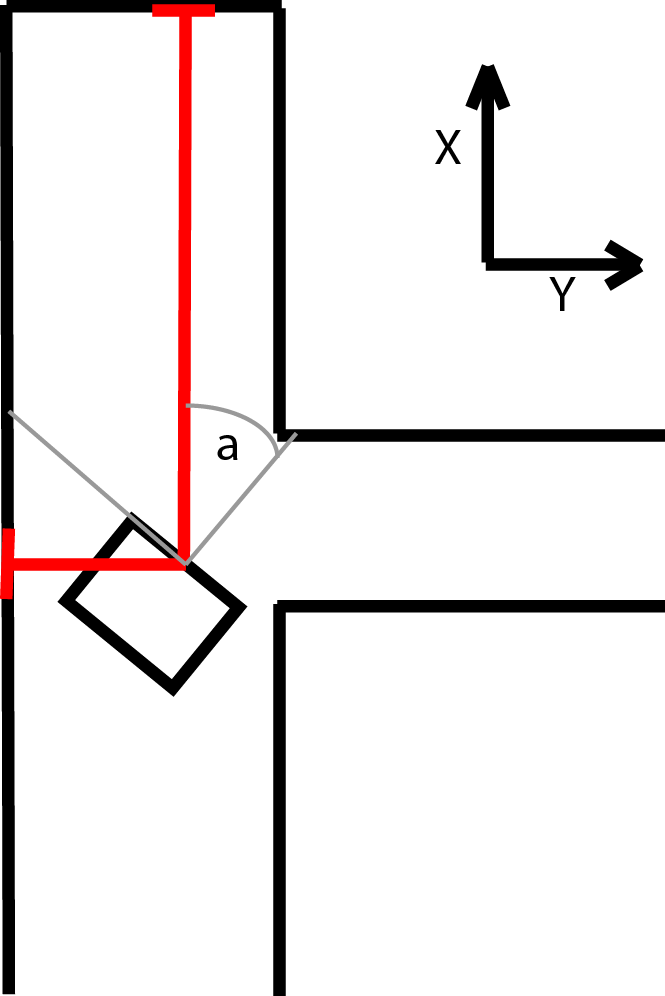
The estimated angle is used to calculate which sensor should point towards the end of the corridor. An interval around the corresponding LRF beam is searched for a local minimum, which should belong to the beam that hits the end perpendicularly. This beam points directly at the end of corridor and is then used to calculate the LRF value for the angle of pico. The difference is calculated between the previous and current distance to the end wall which is the position change for either x or y used in the kalman update. The other position change is calculated in similarly, but in stead of the end of the corridor the distance to the side wall is used. Since it is possible to lose sight of a wall, for instance when driving on an intersection, a safeguard is put in place. If the position change based on the lrf is to big, it is assumed that the LRF data is unreliable for that update cycle and only the odometry data is used. This is done by switching between two R matrices, one of which sets the contributions of the laserdata to zero. In the regular R matrix the contribution of the LRF data is weighed more heavily under the assumption that the LRF is more reliable overall.
Implementation of method
Here the implementation of the method will be briefly discussed.
Interface
Localisation is a separate cpp-file which can be seen as a block. It uses the Scan class data to read sensor data. Also it uses the Drive class to retreive information on the velocity. the variables that are used as arguments are copies and are not used by reference, as they are only needed to calculate the position of the robot. The variables that are only used within the localisation class are ofcourse set to private status. After all necessary blocks are defined in the header file localisation.h , accompanied with the function prototypes, the file localisation.cpp can be properly used. The file consists of 6 functions in total:
- Initializing initial position
- Retreiving LRF-data and converting this into useful X,Y,A data, stored to be used in another function
- Retreiving ODO-data and storing this to be used in another function
- Composing the Z column-vector used in the Kalman algorithm
- Composing the B matrix that is used in the Kalman algorithm
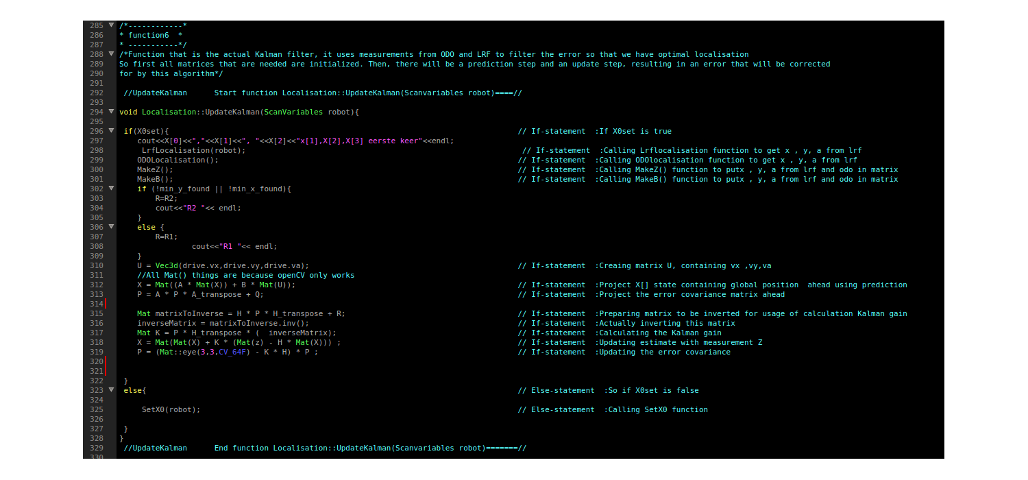
- Function containing the actual Kalman algorithm, which uses the information retreived in the above function to give an accurate localisation
The resulting X,Y,A coordinates are made available to the mapping block for further use. There this info can be used to pinpoint and save nodes, as well as recognizing whether the robot has visited these coordinates before and much more. See the mapping section for further details on this block.
Function 1: initialize position: SetX0()
In this function the position is determined by means of a for-loop that loops over all of ther laser ranges. It determines the minimum range by means of an if-statement. If the minimum range is found, it is stored along with its beam number. This direction is set to correspond to the global Y-direction, and the global angle A is calculated as well, using the beam number. Now the global X-axis is set by using the global Angle. These values are all stored and X,Y,A are initialized.
Function 2: LRF-retreival and conversion: LrfLocalisation()
This function uses the range data to extrapolate the position of the robot. First the angular position A is evaluated. If this angle is larger than pi, or smaller than minus pi, it will be wrapped by subtracting or adding 2 pi respectively. This wrapped angle is used to determine the beam numbers of the current minimal ranges. This is simply done using the following relation:
n_x = X[2]+robot.angle_max / robot.angle_increment; In this equation n_x corresponds to the beam number of the global X-axis and position. X[2] is the global angle A and the other parameters are self explanatory. The range belonging to this beam number is stored. The same procedure is used to determine the Y-data.
In order to create robustness and in order to prevent problems in other function calls, there are some if-statements included to switch axes if necessary. If the beam number n_x is smaller than 4 or bigger than 994, it is one of the outer ranges. If one of these if-statements is true, the beam number n_x will be changed. We switch from the positive to negative axis or the other way around, by adding pi to the angle. This way, the axis can not get out of sight of the robot. Simple boolean expressions are used to notify the system whether the positive or negative axis is being tracked. This is important because it changes whether distances should be counted negative or positive. This system using axis-switches is incorporated, because there is no assumption made regarding initial position. It should be able to determine an axis to track, regardless of the initial angle of the robot in the maze.
Next the values of the ranges are checked between n_x-5 and n_x+5 using a for-loop. If a minimum range is found it is stored. However, if the minimum value lies on the outer bounds of the loop, or if the difference is too small (noise) , then no minimum is found. This is done for both the x- and y-direction.
Finally, using the laser distance in x- and y-direction, the difference is range is calculated with the previous function call. These differences represent the movements made between function calls, and therefore the difference in position. Every function call, the differences in each direction are added to the total of differences calculated in previous calls. These variables therefore represent the global X,Y and A position.
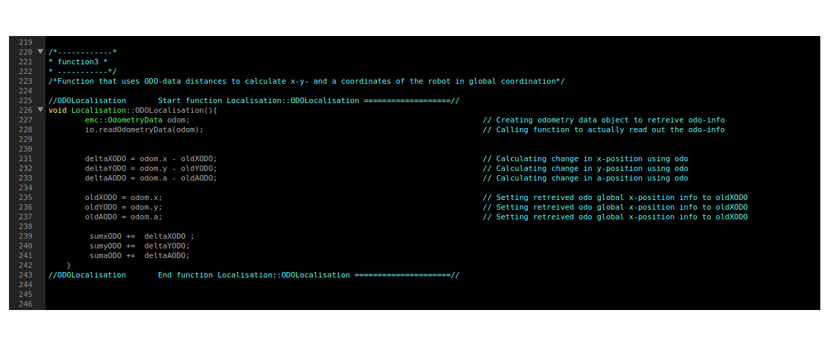
Function 3: ODO-retreival: ODOLocalisation()
This function creates an odometry object and reads the odometry data from the io-layer. It starts with an initial X=0,Y=0,A=A_init . It calculates the differences each time the function is called. So if the x position is 5 meter, and the next function call it reads 5.2 meter, then the difference equals the recent reading minus the old reading. The differences are stored, as well as the old position and the sum of the differences (actual position). This info is to be used by the other functions that need it in the file.
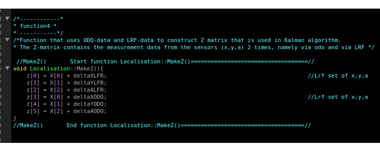
Function 4: Making Z: MakeZ()
Z is a 6-entry column vector. Every time it is called, it will update the entries as follows: The first three entries (corresponding to X_lrf,Y_lrf and A_lrf respectively) equal their global position plus the difference in position calculated in the LRF retreival function. The latter three entries correspond in the same manner to their odometry counterparts. These second X_odo,Y_odo and A_odo are updated in the same manner, but using the difference in odometry instead of LRF. The odometry differences are calculated in function 3. Now the Z-column vector is ready to be used by the Kalman filter.
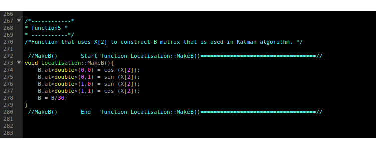
Function 5: Making B: MakeB()
This function simply constructs the 3x3 matrix B that is used in the Kalman algorithm. The first two rows concern the X-and Y-position. Therefore the first row consists of the cos([X[2]) and the sin(X[2]) and zero respectively. Ofcourse the mirror is true for the Y-position. So the second row consists of sin([X[2]) and the cos(X[2]) and zero respectively. The third row contains zero entries for the first two columns, and a value of 1 for the angular entry.
Function 6: Kalman filter: UpdateKalman()
Technicalities and solutions
Problems with Localisation block
====Alternatives: ====