Embedded Motion Control 2019 Group 4
This is the CSTWiki page for group 4 of Embedded Motion Control 2019.
Group members
| Marcel Bosselaar | 0906127 |
| Ruben Sommer | 0910856 |
| Jeroen Setz | 0843356 |
| Bram Grolleman | 0757428 |
| Martijn Tibboel | 0909136 |
Deliverables
Escape Room
The following ideas are used for the excecution of the Escape room.
Escape Room - Plan
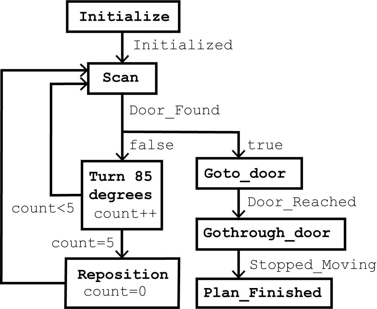
The initial strategy that is formulated is as follows:
This plan is updated to gain more insights and control over the different situations that can happen.
[PLAATJE]
Escape Room - Exit recognition
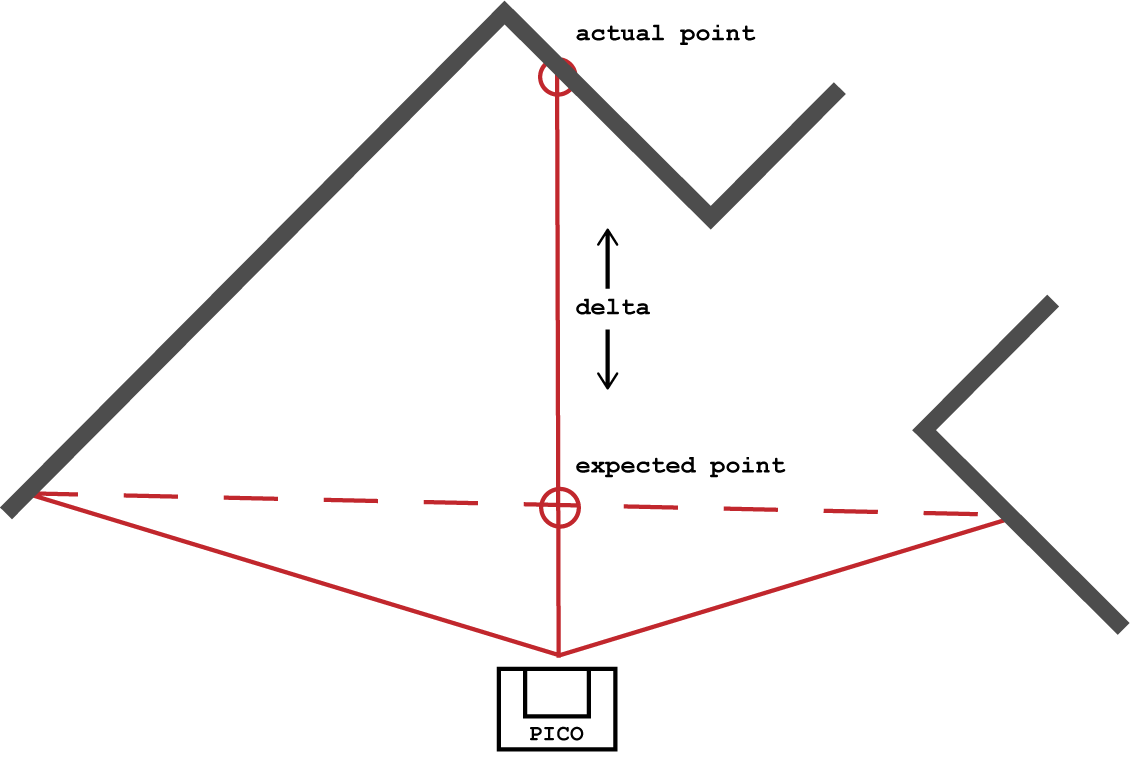
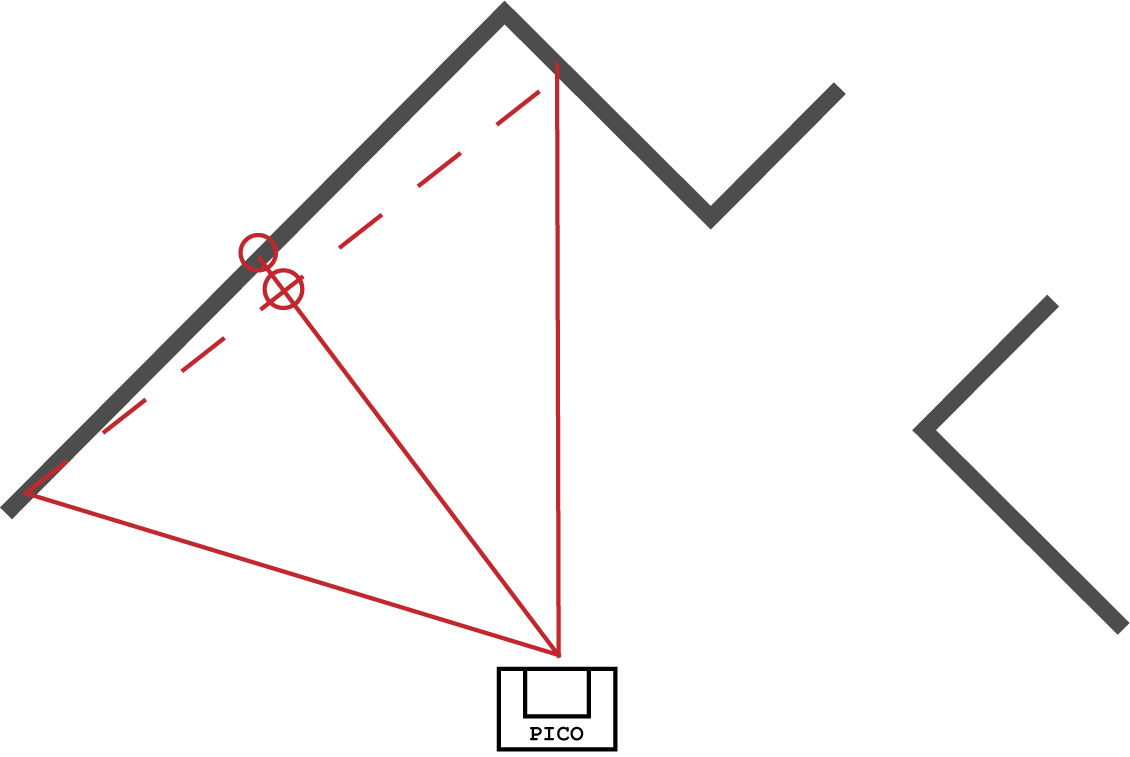
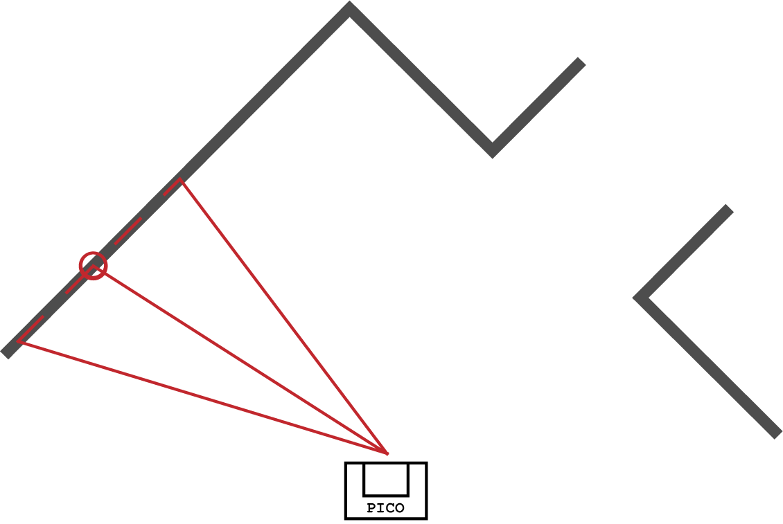
Firstly walls are created from the lrf data. Next, these small walls are merged into large walls. For this, the 'split and merge' method is used as shown below.
-
Example first step
-
Example second step
-
Example third step
Then the corners are recognized. The 2 different kind of corners are recognized and from the right kind of corners the exit is generated. This is visualised below.

At last, the center point of the exit is calculated together with a point in front of this center point. This point in front is sent to the movement part of the PICO.
Escape Room - Finite state machine
A finite state machine is introduced in order to maintain control over what is happening at all times.
After the challenge, an alternative FSM was thought of that reduces the number of states required and vastly improves accuracy.
-
Diagram of the finite state machine used in the escape room competition.
-
Diagram of an improved FSM, thought of after the competition.
Escape Room - Testing
The following testing dates are set. Also the goal of each testing date is put behind in order to stay on track of the global planning of the project.
- PICO Test 1 (2019-05-08) --> Goal: have PICO detect the exit, and perform simple motion towards it.
- PICO Test 2 (2019-05-13) --> Goal: use a more advanced algorithm to detect and move.
- PICO Test 3 (2019-05-16) --> Goal: Test improvements done based on competition results. If available, test ideas that were previously generated but would only be useful for the final competition.
Escape Room - Competition
In the escape room competition, we were potentially the team that had the highest high and the lowest low.
The algorithm we had designed worked perfectly and very quickly. The door was found as soon as it came into view, and PICO decided to move toward the correct location in front of the door. The door was then immediately found again, and PICO's position in front of the door was made more accurate. Then, the exit of the hallway was detected immediately, and PICO drove towards its end goal.
However, due to the fact that we had not managed to implement the odometry into PICO, distances traveled were around 30% too short, meaning PICO stopped well before the detected end of the exit hallway. In addition, telling PICO to drive straight didn't actually make it drive straight, making it graze the wall.
The first improvement we will need to make is the odometry, as we're confident PICO would have exited the room within 30 seconds if it actually was were it thought it was. Secondly, we should use the laser data more frequently, and create new plans during movement to keep things moving in the right direction. Improving the finite state machine to use fewer states and being more circular might also be a good addition.
Hospital Challenge
The following section explains the different functions build and used in the hospital challenge.
Hospital Challenge - State machine
Due to the hospital challenge requiring different functionality from the escape room challenge, a new finite state machine was developed, visible below.

Explanation
In this state machine, there is once again an initialization state, called init. Once PICO has been initialized, which is checked by grabbing LRF and odometry data and seeing whether it is correct, the event initialized occurs, and the state
Implementation
The state machine as described above has been implemented in the software as an enum type variable for the events and for the states. This type of variable can only have the values of the states/events, declared in its generation.
The monitor function is the only function that can alter the states, and it will do so based on the events generated by the other functions. For instance, when the event goalSelected is thrown, by way of the variable E having value goalSelected, the monitor will change the state to goalPlan, by way of changing variable FSM to goalPlan.
The perception, planning, and control functions will then display different behavior depending on what the value of FSM is. This is achieved by creating multiple successive if-loops that describe the behavior in a certain state or states.
Hospital Challenge - Localization
For the hospital challenge localization is key to achieve goals. If everything works but you don't know where you are it is going to be a mess. The idea is to update the localization every time the robot needs to make a new path with the path planning. In between two setpoints of the path, the odometry is used to know the current location and this is assumed to be 'good enough'. When something goes wrong and it is not enough, the state machine compensates, because the robot goes to a 're-planning' state, where it also updates the location again. This way it is never a problem if the accuracy of the localization is a bit off.
Point matching
The idea that is used for localizing PICO's location is as follows.
When PICO is being initialized, a calculation is done over the map information. All corners are specified with the right corner type 'inside' or 'outside' corner, wich is also done for the LRF data as explained in the escape room challenge. For all corners of the map is the distance between the point and all other points calculated for use in the future.
Within the localization script a loop is made through all corners of the map and all corners that are specified in the LRF data. A point of the LRF data is checked if it has the same kind of corner as the map point. If that is true, another point of both data sets is checked if this has the same kind. When this holds, a distance is calculated between the points of the LRF and then checked if this distance is near the distance that it should be compared to the map. (which is stored in the beginning) Summarizing, this means that a wall with 2 points of the LRF data is checked if it is suits to be fitted to a wall of the map.
Next, this is done for another three walls, while aborting if one of the statements does not hold. This reduces the amount of possibilities of the best fit and the possible fits are stored in an array. After this, the script uses the stored fits to calculate a location of PICO in the map with the given distances from the LRF corners that are fitted in the fits. The different that come forward are analysed on the amount of occurances and unfeasible locations (outside the map for example) are removed from the possibilities.
From the locations that are found a mean location is calculated together with the guess (from the odometry data) where PICO possible could to obtain the final location of PICO. Accordingly to the location of PICO the map is translated and rotated in order to fit the map over the LRF data. This way the planning can be done easier, because it is assured that PICO is at the origin of the plot.
A problem occured while making this way of localizing. The localization had a lot of 'unwanted' locations, so that is why the above filters were added. This solved the problem, but still a offset remained within the localization. Later on it appeared to be a problem within the shifting of the map, because we were using multiple coordinate system which made reasoning pretty hard. In the beginning we thought it was the uncertainty of the found points that gave this offset, that is why we also looked at other localization options. Which in the end, turned out to have the same problem.
Alternatives
- Cabinet and Door recognition
- Particle filter
Hospital Challenge - Path planning
Path planning is defined here as finding a way from point A to B based on a known map while avoiding obstacles on this map. In general there are four different approaches to path planning for mobile robotics:
- Cell decomposition
- Divide the map into a grid and define obstacles as cells which can not be used for movement. Then an algorithm as A* or Dijkstra can be used to find the (optimal) path from A to B.
- Potential fields
- A map is converted to a potential field map in which obstacles have high values and free space low. This way a path from A to B can be created which follows the lowest potentials.
- Sampling based
- A sampling based algorithm finds points in the free space of a map and tries to connect them. Then a path is found from A to B following these points. Examples are a Rapidely-expanding Random Tree (RRT) or a probabilistic roadmap.
The requirement set for a path planning algorithm was to avoid a grid (to prevent scalability issues and limited cell resolution) and potential fields (as followed from the Do's and Don'ts lecture). Therefore one candidate remained: sampling based. The choice was made to use a RRT algorithm as is seemed easier to implement compared to a probabilistic roadmap.
Rapidly-expanding Random Tree algorithm
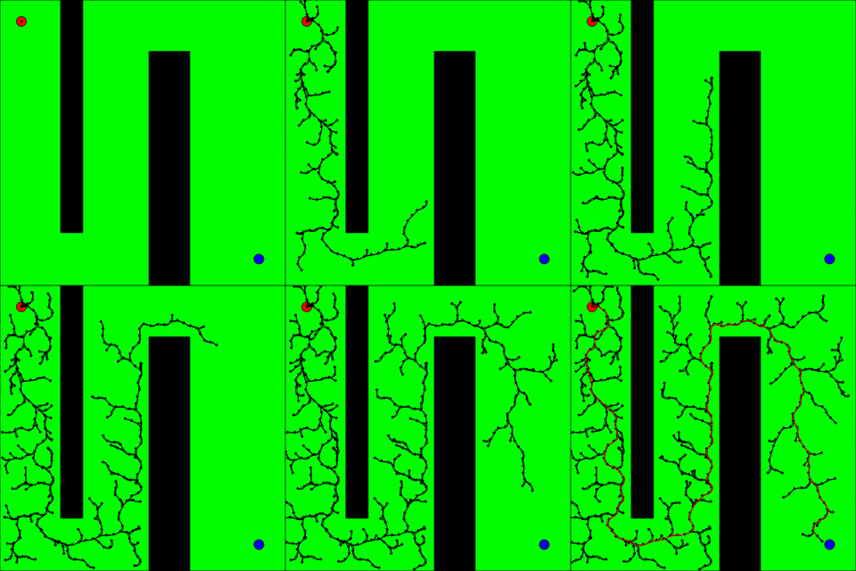
A RRT algorithm starts with a root node. In this case the initial position of PICO. Each iteration a random point is created in the space of the map. The closest node of the tree to the random point is chosen to extend the tree in the direction of the random point. The connection of the newly placed node will be checked for validity (i.e. not colliding with obstacles on the map). This way the random tree will eventually span the complete free space. The algorithm terminates if the goal point B is reached with the tree. An open-source existing algorithm is used which creates a basic random tree. This is modified to work with our software. Two (major) additions are done to the existing algorithm.
RRT end point bias
To ensure a quick convergence of the tree towards the end goal (point B), an endpoint bias is used. This means that every few iterations the algorithm does not use a random point is space but the end goal. This way the tree will be extended in the direction of the goal. This proved to achieve a much faster algorithm which required a lot less iterations to find a path. The end point bias may to be too large (i.e. take every other random point as the end point) as the algorithm can get trapped in corners between obstacles.
RRT path splitting
A drawback of the RRT algorithm is that it will find a path which is generally not optimal. To optimize the found path, a splitting algorithm is used similliar to the splitting algorithm used to find walls in LRF data. It first tries to connect the start and end point of the path to see if it can be connected with a straight line without colliding with obstacles. If this fails, the check is done using the middle point of the path. This is done recursively to optimize the path. In the worst case scenario the original path will be retrieved again. The RRT splitting method showed to create nice straight lines between all points on the path, this still does not create an optimal path, but an optimized version of the original found path.
Hospital Challenge - Movement
Hospital Challenge - Global movement
Hospital Challenge - Local movement
Hospital Challenge - Obstacles
Hospital Challenge - Obstacle recognition
Hospital Challenge - Obstacle avoidance
Hospital Challenge - Software Architecture
Hostpital Challenge - Testing
Hospital Challenge - Competition
- Conclusion
