Mobile Robot Control 2024 Robocop

Group members:

Caption

Name	student ID
Matijs van Kempen	2060256
Luc Manders	1729225
Marc Quelle	2044749
Marijn Ruiter	1489496
Luke Alkemade	1581643
Arif Ashworth	1544632
Abhidnya Kadu	1859234

Exercise 1

Method 1

Screenshot of final result for Method 1.

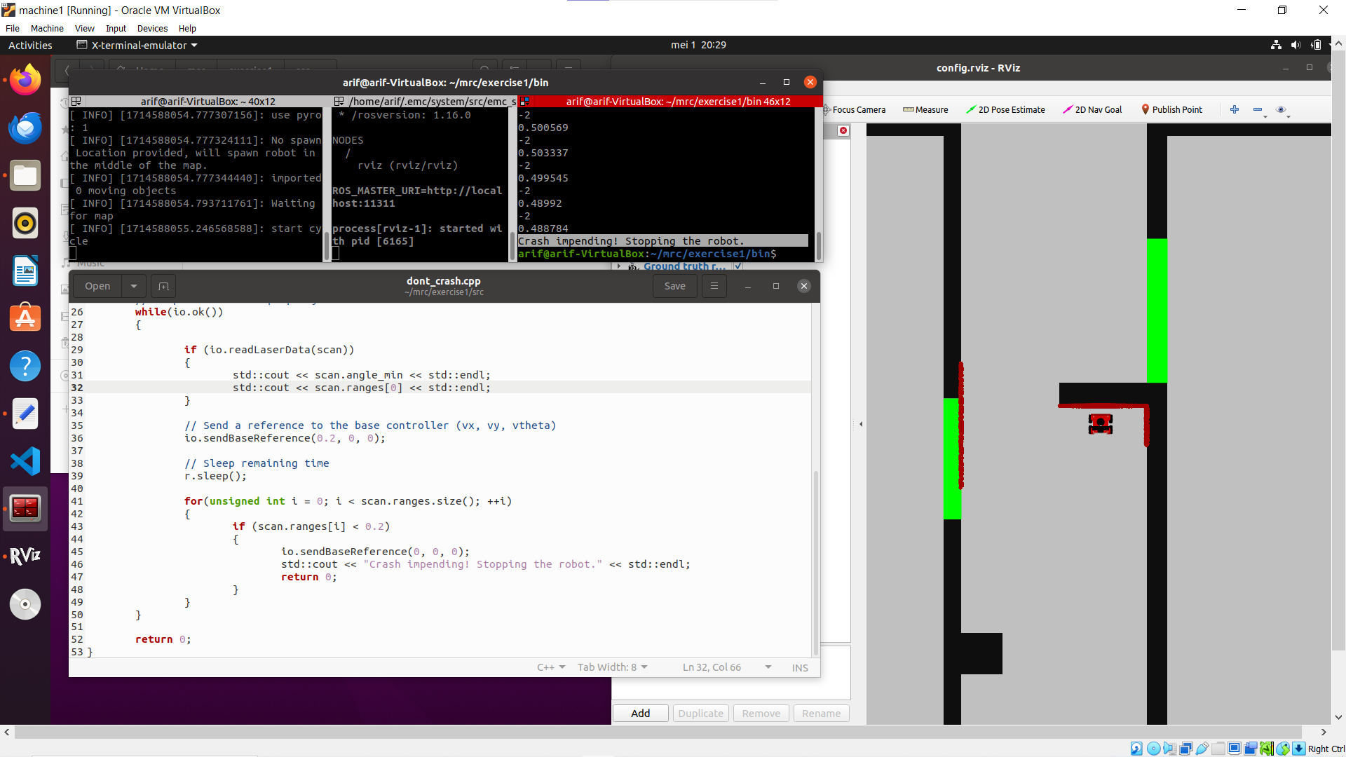
In this method the LaserData struct is used to track the measured distances from the walls to the robot. To make the robot drive forward the sendBaseReference command is used, and the robot moves in the x direction at a speed of 0.2. Once it reaches the wall in front of it and the range values drop to below 0.2, motion is halted and a message is printed to the screen before exiting the program.

Some experimentation was done to test different speeds and thresholds for the stopping range values. When the speed was higher than the stopping range value the robot would actually crash into the wall first before stopping, and if it was lower then the robot would stop slightly farther away from the wall. However, this only seemed to be the case when the stopping value was very low (e.g. 0.1), but increasing it to 0.2, for example, allowed the speed to be increased to 0.4 without any crashing.

Exercise 2

Method 1

Method 1 on Map 1.

Method 1 on Map 2.

The previously described method was tested on the two provided maps with input speeds of (0.3, 0, +-0.3) and a stopping value of 0.2. With both maps the robot successfully came to a stop before crashing, although it struggled when driving into a corner and stopped much closer to the wall than it did in previous tests.

Local Navigation

Dynamic Window Approach

The approach

The approach can be divided in the following sequential steps:

1. Calculate the union between the Possible (angular) Velocities (Vs, Ws) and the Reachable (angular) Velocities (Vd, Wd)
   • EXPLAIN HOW
2. Iterate through the discretized values (v, w) of the union of Vs, Vd and Ws and Wd:
   1. Calculate the Admissable (angular) Velocities (Va,Wa) using v and w
      • EXPLAIN HOW
   2. Check if v and w are also in Va and Wa, if this is the case:
      • Calculate the optimization function value. If this value is higher than the previous optimization value, set the current v and w to v_final and w_final
        • EXPLAIN HOW
3. Return v_final, w_final

Our approach for the Dynamic Window Approach (DWA) is that we first make a list of samples that fit inside the possible velocity limit (Vs) and reachable velocity and acceleration constraints (Vd). After which we

Questions

1. What are the advantages and disadvantages of your solutions?

Advantages:

1. By constantly calculating possible trajectories it is able to avoid dynamic and static obstacles.
2. By including the robot acceleration and deceleration constraints it ensures for a smooth navigation without abrupt movements.

Disadvantages:

1. DWA may get trapped in a local minima.
2. There is a high computational load in calculating the multiple trajectories in real-time

2. What are possible scenarios which can result in failures?

1. Like mentioned in question 1 DWA can get trapped in a local minima.
   • Solution: Include the global planner so it doesn't drive into a local minima
2. We also encounter some problems when the robot is driving to a straight wall and can't decide with direction to take. (see video: https://gitlab.tue.nl/mobile-robot-control/mrc-2024/robocop/-/blob/main/videos_and_photos/dwa_straight_wall.mp4)
   • Solution: Increase Ks and decrease Kh so the robot is less constrained to drive directly towards the goal.

3. How are the local and global planner linked together?

Vector Field Histograms

The approach (main idea)

The idea of the VFH is to create a vector field histogram from the laserdata of the robot. the VFH is a graph with angle on the x axis and likelihood of a blocking object on the y axis. When the y axis is below a certain threshold, we know that the robot can drive unobstructed in corresponding direction. We can now choose the angle that is unobstructed and closest to the wanted goal. In our approach of the circa 1000 laser be shapams 100 histogram bins are created. the circa 10 beams per bin get inversely (1/distance) added. This creates higher values of bins where there are obstructions.

Questions

1. What are the advantages and disadvantages of your solutions? the algorithm is computationally efficient. the laser scan data gets looped through a few times (collecting laser data, making the VFH from the laserdata, optional filtering of the VFH, choosing the best angle). This way the algorithm updates the robot without to much delay from the real time data. a disadvantage of the algorithm is that it doesn't account well for size of the robot. even when inflating the walls in software the casting of the laser beam make it unpredictable if you actually drive aground a wall instead of next to the wall. It does drive itself around but the path isn't always optimal.
2. What are possible scenarios which can result in failures?the algorithm will not navigate mazes itself. If there are too much obstructions the robot could get stuck between a few points. When entering for example something like a U shape that is larger than its viewing window. The robot will enter the hallway thinking it's is free, when seeing the end walls it will turn around until it doesn't see the wall anymore. At that point the robot will again turn around to get stuck in a loop.
3. How would you prevent these scenarios from happening?By integrating a good global planner the robot already won't go into these U shapes. If it finds itself stuck on a point that a global map didn't see the robot can report this back and again find a global route that can be locally navigated.
4. How are the local and global planner linked together?

Global Navigation

Questions

1. How could finding the shortest path through the maze using the A* algorithm be made more efficient by placing the nodes differently? Sketch the small maze with the proposed nodes and the connections between them. Why would this be more efficient?
2. Would implementing PRM in a map like the maze be efficient?
3. What would change if the map suddenly changes (e.g. the map gets updated)?
4. How did you connect the local and global planner?
5. Test the combination of your local and global planner for a longer period of time on the real robot. What do you see that happens in terms of the calculated position of the robot? What is a way to solve this?
6. Run the A* algorithm using the gridmap (with the provided nodelist) and using the PRM. What do you observe? Comment on the advantage of using PRM in an open space.

Upload screen recordings of the simulation results and comment on the behavior of the robot. If the robot does not make it to the end, describe what is going wrong and how you would solve it (if time would allow)

Upload video's of the robot's performance in real life (same as simulation videos), and comment the seen behavior (similar to the previous question).