Mobile Robot Control 2020 Group 8

Group information

Group Members

Name	Student Number
J.J.W. Bevers	0904589
J. Fölker	0952554
B.R. Herremans	0970880
L.D. Nijland	0958546
A.J.C. Tiemessen	1026782
A.H.J. Waldus	0946642

Meeting Summaries

A logbook with a summary of the contents of each meeting is documented and can be found here

Course description

Introduction

Figure 1: PICO.

As is proven during the current situation concerning the COVID-19 pandemic, our healthcare system is of high importance. However, there are shortcomings for which an efficient solution is required. At the time, the hospitals are occupied by many patients. Therefore, doctors and nurses have limited time for human-to-human contact with patients. By automating simple tasks, doctors and nurses have more time for contact with patients. An option is to use an autonomous embedded robot to assist in the everyday tasks such as getting medicine, moving blood bags or syringes and getting food and drinks. During this course, software for such an autonomous robot is developed. The goal is to complete two different challenges in a simulated environment: the Escape Room Challenge and the Hospital Challenge.

PICO

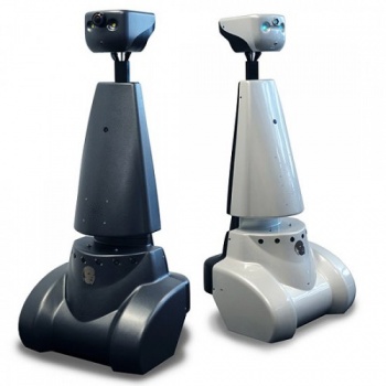
The mobile robot used is called PICO and is shown in Figure 1. PICO consists of multiple components. This year's edition of the course will be completely based on the PICO simulator (as developed by the project team) and will, thus, not contain implementation of the software on the actual robot. Only the relevant components for simulations are, therefore, briefly explained. For actuatation purposes, PICO has three omni-wheels which make for a holonomic base. A Laser Range Finder (LRF) is used by PICO to scan its surroundings, providing PICO with distance data. Furthermore, the wheel encoders data is used to keep track of PICO's translations and rotation (odometry).

Figure 2: Example of the map used for the Escape Room Challenge (left) and the Hospital Challenge (right).

Escape Room Challenge

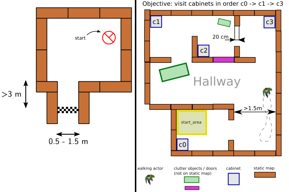
The goal of this challenge is to navigate PICO, through a corridor, out of a rectangular room of unknown dimensions without bumping into walls. An example of an environenment map that might be encountered during this challenge is shown on the left side of Figure 2. PICO has an unknown initial position within this room. Thus, PICO first needs to detect and recognize the exit. When the exit is found, PICO has to exit the room as fast as possible by moving through the corridor. The challenge is finished when the rear wheels of PICO cross the finish line entirely. In the section Escape Room Challenge, the approach is explained in more detail. Here, the algorithms used and its implementations are explained. Moreover, the results of the challenge are shown and discussed.

Hospital Challenge

This challenge represents an example of the application of an autonomous robot in a more realistic environment. In this challenge, PICO has to operate in a hospital environment. The environment will consist of multiple rooms, a hallway and an unknown number of static- and dynamic objects. In the rooms, cabinets are present that contain medicine. In this challenge, PICO will first need to recognize its initial position in the known environment. Next, PICO has to plan a path to various cabinets in a predefined order, representing the collection and delivery of medicine. When executing this path, PICO needs to prevent collisions with walls, and static- and dynamic objects. An example environment is shown on the right side of Figure 2. In Section Hospital Challenge, more information will be provided.

Design document

In this section, an adapted version of the design document is found which incorporates received feedback. The original design document can be found in Section Deliverables. The design document serves as a generic document applicable to both challenges. The functions listed are an initial guess of what is thought to be needed before actually working on the software. When producing the software, the actual functions arose. These functions are listed and explained in the Sections Escape Room Challenge and Hospital Challenge.

Requirements and Specifications

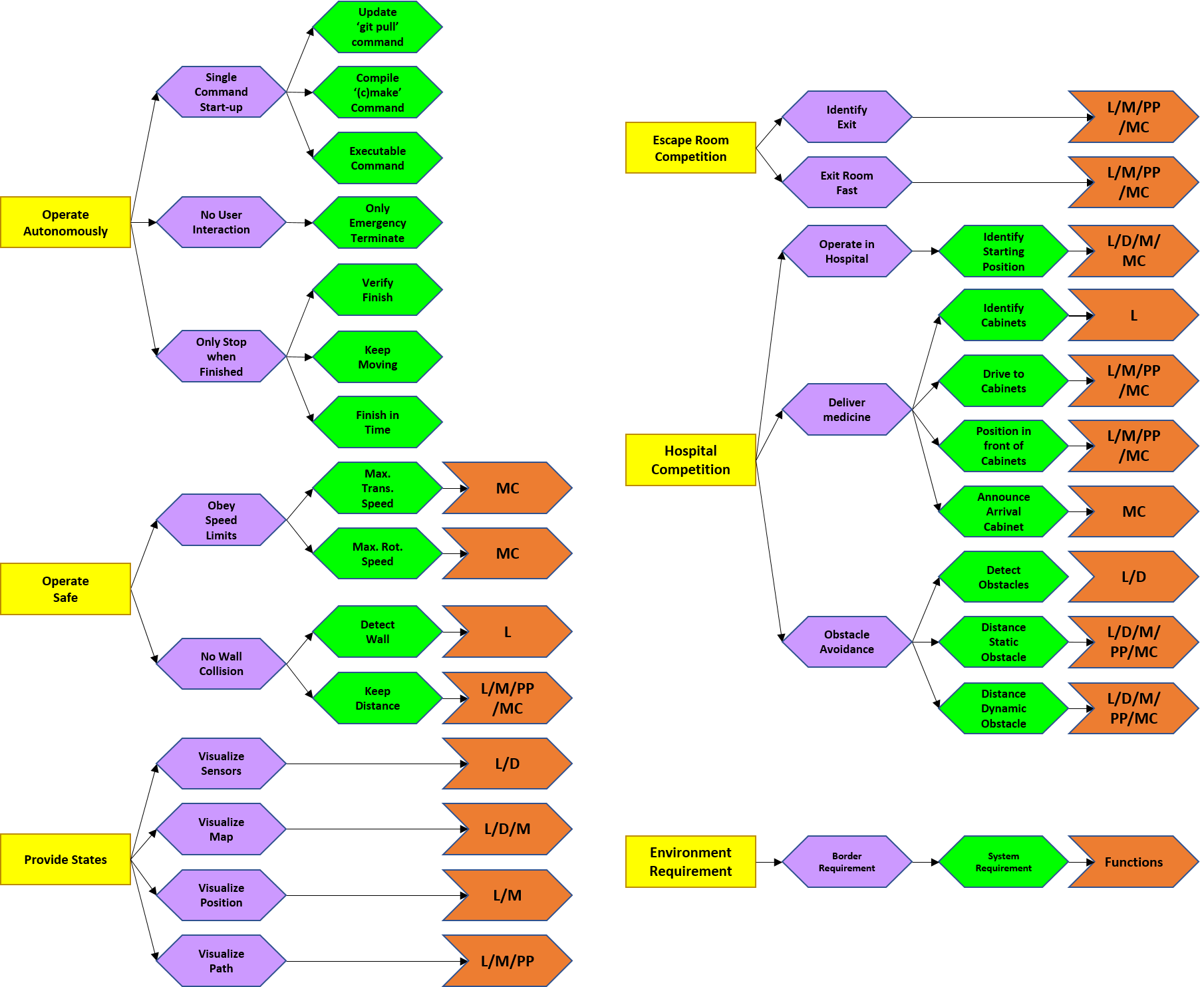
A distinction is made between general and competition specific requirements. Three stakeholders are considered: the hospital employees, the patients and the software engineers. In ascending order, the requirements are subdivided into environment requirements, border requirements, system requirements and function types. Five functions types are introduced: Localization(L), Detection(D), Mapping(M), Path Planning(PP) and Motion Control(MC). These are elaborated in the next section. The requirements are shown in Figure 3 and elaborated below. Note the legend located bottom right. First, the five environment requirements will be discussed in more detail. Even though the environment requirements are shown as separate parts, they do relate to each other. The first three environment requirements correspond to the functionality of PICO and are thus relevant for both challenges. The fourth and fifth environment requirement are specifically defined for the Escape Room- and Hospital Challenge, respectively.

• PICO should operate autonomously: No interaction is allowed, unless an emergency stop is needed. To start the software, the ’git pull’ command is used to update, the ’cmake’ and ’make’ commands are used for compiling and one executable is used to start execution.

• PICO can only stop executing when its task is finished: Therefore it must be able to verify when it is finished. Also, PICO cannot be stationary for 30 consecutive seconds and the task must be finished in time. PICO should operate safely. In order to do so, it must obey speed limits. A maximum transnational and rotational speed of 0.5 m/s and 1.2 rad/s, respectively, are set.

• PICO can not bump into walls: Therefore, PICO should be able to detect walls and keep a certain distance. PICO should provide information on its state. Therefore, PICO should visualize its sensor data, produce and visualize a map and its current position and finally visualize its produced path.

• PICO should finish the Escape Room Competition: To succeed, PICO must be able to identify the exit and it should exit as fast as possible. A strategy is explained in the next section.

• PICO should finish the Hospital Competition: PICO should deliver medicine. Therefore, PICO must recognize cabinets, drive to them, position in front of them facing towards them and afterwards produce a sound signal. PICO should operate in the hospital environment. Therefore it must recognize its (initial) position in the provided map. Finally, PICO should not bump into static or dynamic objects. Thus PICO should detect an object within a 10 meter range and the distance between PICO and a static or dynamic object must be at least 0.2 m and 0.5 m respectively.

The hospital employees are involved in the first, second and fifth requirement, the patients in the second and fifth and the software engineers in the first, third and fourth.

Figure 3: The general requirements (left), the competition specific requirements and legend (right).

Functions

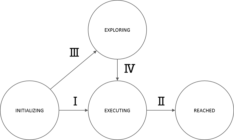
The finite state machine displayed in Figure 4 depicts the designed behavior of PICO, allowing it to complete the two challenges. The states are:

• State I - Initializing: PICO performs an initial scan of it’s surroundings and maps this data to find its position on the map. It is possible that insufficient information has been gathered to do this when, for instance, all objects are out of reach of the laser range finder.

• State II - Exploring: An exploration algorithm such as a potential field algorithm or a rapidly expanding random tree algorithm is used to explore the environment further. When PICO’s position within the map is known and the exploration algorithm has been executed for T seconds, the transition to State III occurs.

• State III - Planning: After PICO has localized itself on the map, enough information has been gathered to compute a path towards a target. An algorithm is used to compute a state trajectory, that is then translated into control actions.

• State IV - Executing: During this state a control loop is executed which controls PICO towards the reference coordinates (x,y) by measuring position and actuating velocities. When PICO runs into an unexpected close proximity object, the state is transferred to State V. When PICO runs into an unexpected distant proximity object, the state is transferred to State III, such that a new path can be planned before PICO arrives at this object.

• State V - Recover: During the recover state, PICO has encountered a close proximity object which it did not expect. PICO then immediately stops and when completely stopped, it transits to State II, such that the exploration algorithm can move PICO away from this unexpected object for T seconds. The loop (State II, State III, State IV, State V) can be executed repeatedly and can be counted, such that T increases when more loops are encountered.

• State VI - Reached: After the path execution has been finished and PICO has reached the end of the path, PICO stops moving as it has reached its target location.

Figure 4: Finite State Machine

FUNCTION	DESCRIPTION
Localization
InitialScan()	PICO makes a rotation of 190 [deg] to get a full 360 [deg] scan of the environment
GetMeasurement()	Read out the laser range finder sensor data
Detection
ProximitySense()	Detects if an unexpected object is in close proximity
DistantSense()	Detects if an unexpected object is in distant proximity
Mapping
UpdateMap()	Write measured data to Cartesian 2D world map used by path planner
UpdatePotField()	Write measured data into potential field map used by potential field algorithm
GetMap()	Retreive current 2D carthesian world map and (x, y) position of PICO
GetPotField()	Gets gradients from the potential field
Path Planning
GetGoal()	Retrieve Cartesian coordinates of the goal (xg, yg) with respect to the map
PlanPath()	Path planner algorithm using the 2D world map to plan a state trajectory (x, y array)
ComputePotState()	Uses gradients from potential field as input, to compute a state reference ẋ, ẏ, \dot{θ}
ReadPath()	Get current (x, y) goal of path array
Motion Control
Move()	Send position reference (x, y, θ) to PICO. Contains position control loop
StopMoving()	All movements of PICO are stopped: ẋ, ẏ, \dot{θ} = 0
FullRotation()	PICO makes one full rotation
ExecutePath()	Translates (x, y) path reference into controller action for calling Move(). Loop over all (x, y) to achieve position reference tracking

Software Architecture

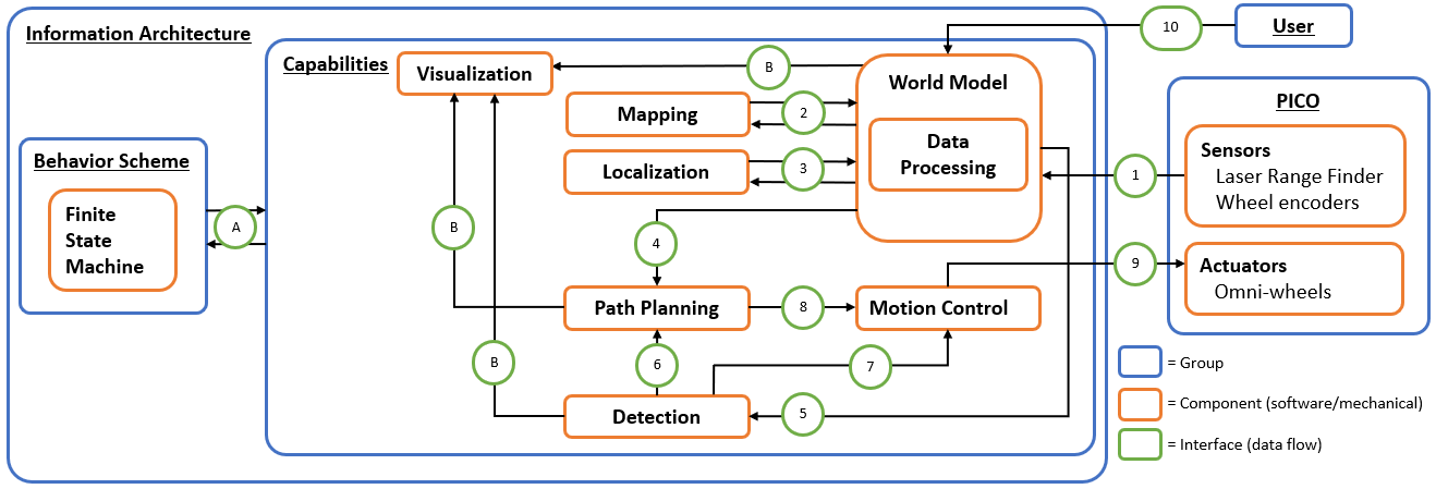
The proposed information architecture is depicted in Figure 5. It shows a generic approach, so note that a specific challenge may require additional functionalities and interfaces. Between the software and mechanical components, information is shared via interfaces marked in green and labeled with an arbitrary number or letter. These interfaces dictate what information is set by which component and what information is shared, and among which components. In the central section, this schematic overview visualizes what capabilities are intended to be embedded in the software. Firstly, interface 10 represents the data received from the user, which may include a JSON file with a map and markers, depending on the challenge. On the right, interface 1 between PICO (including the provided software layer) and the designed software shows the incoming sensor data, i.e. structs with distance data from the Laser Range Finder (LRF) and odometry data based onthe omni-wheel encoders. This data is (possibly) processed and used to map PICO’s environment (mapping), to estimate PICO’s position and orientation (localization), and to detect static/dynamic obstacles (detection), via interfaces 2, 3 and 5. This knowledge is stored in the world model,serving as a central data-base. Via interface 4, a combination of the current map, PICO’s poseand the current (user-provided) destination is sent, to plan an adequate path. This path is sent over interface 8, in the form of reference data for the (x,y,θ)-coordinates. The motion controlcomponent will then ensure that PICO follows this path by sending velocity inputs over interface 9. Simultaneously, the detection monitors any static/dynamics obstacles on the current path online. If this is the case, interfaces 6 and 7 serve to feed this knowledge back to either the path planning component to adjust the path or directly to motion control to make a stop. On the left, interface A between the behavior scheme and the capabilities shows that the high-level finite state machine manages what functionality is to be executed and when. Interfaces B represent the data that is chosen to be visualized to support the design process, i.e. the visualization serves as a form of feedback for the designer. The information that is visualized depends heavily on the design choices later on in the process and, therefore, this will not be explained further.

Implementation

The components described above are intended to be explicitly embedded in the code through the use of classes. The functionality that belongs to a certain component will then be implemented as a method of that specific class. At this stage of the design process, the specific algorithms/methodsthat will be used for the functionalities are not set, but some possibilities will be mentioned here. Simultaneous mapping and localization (SLAM) algorithms, based on Kalman filters or particle filters, could be used for the mapping and localization components. Moreover, for path planning, Dijkstra’s algorithm, the A* algorithm or the rapidly-exploring random tree algorithm can be used.For motion control, standard PI(D) control, possible with feedforward, can be used to track the reference trajectory corresponding to the computed path. Additionally, for detection, artificial potential fields can be used to stay clear from obstacles.

Figure 5: Software Architecture

Escape Room Challenge

In this section, the strategy for the Escape Room Challenge is discussed, as well as the algorithms that are used. The software for this challenge can be roughly divided into three main parts: the finite state machine, the potential field algorithm and the exit detection algorithm. These will be covered next.

Finite state machine

A Finite State Machine (FSM) that describes the robot's behavioral scheme is designed, forming the basis of the software architecture. The FSM describes which states can be reached from a certain state, given the response of that state to some input. For the Escape room challenge, a total of four behavorial states are implemented as can be seen in the figure down below. The states of the FSM are defined as followed:

Initializing: PICO performs an initial scan of it’s surroundings and searches for the exit. If the exit is detected, the detection algorithm will place a node in the middle of the beginning of the exit corridor and the state transitions to the executing state. If the exit is not detected after the first rotation of 360 degrees, the state transitions to the exploring state.

Exploring: A potential field algorithm is used to explore the environment further. Untill the detection algorithm has located the exit, PICO will drive in a straight line untill it reaches a wall. When a wall is reached, the repulsive field of the wall becomes tronger than the atrractive field that is placed 1m in front of PICO, making the robot rotate away from that wall. This movement continues untill the exit is detected.

Executing: In the executing state, an attractive field is placed on the location that the detection algorithm has indicated as a target. The vector that follows from the combined attractive and repulsive field is translated into translational and rotational velocities, which are used as input for the robot motion. Multiple targets can be identified in the executing state, for example the beginning of the exit corridor and the end of the exit corridor. When PICO has reached the last target and it no longer detects any walls, the state transitions to the reached state

Reached: After the path execution has been finished and PICO has reached the end of the path, PICO stops moving as it has reached its target location.

Figure 4: Finite State Machine

Potential field algorithm

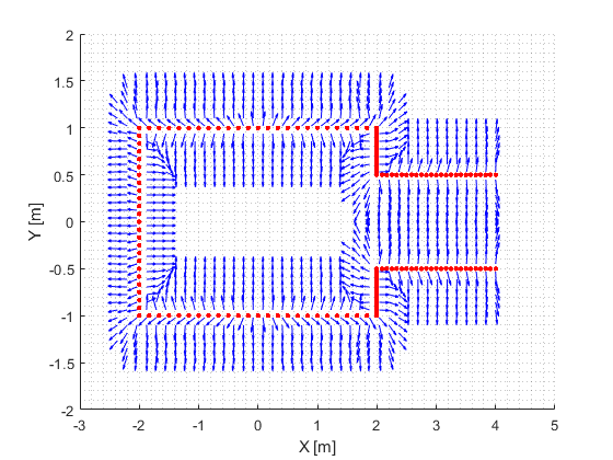
During the Escape Room Challenge, the direction and magnitude of the velocity of PICO is guarded by the potential field algorithm. The potential field within a mapped environment consists of a rejective field and an attractive field. An example of a gradient field from the rejective field is shown in Figure 6. For the Escape Room Challenge however, it is chosen to not use a worldmap as this would unnesesarily overcomplicate computations. Therefore the rejective field vector at PICO’s current position is computed based on all current LRF data, such that the gradient with respect to PICO’s local coordinate frame based on its current measurements is computed. For the attractive field, the current goal relative to PICO’s local coordinate frame is required. This goal is provided by the exit detection algorithm. The vector corresponding to the gradient of the attractive field is computed by means of a convex parabola in the XY-plane with respect to the local coordinate frame of PICO, which has its minimum at the goal relative to PICO’s local coordinate frame. Both the rejective and the attractive field vectors are normalized to have a magnitude of 1. This avoids the effect that the rejective field is stronger when PICO observes more datapoints at a certain moment, which could give a distorted effect in the magnitude of the rejective field gradient vector.

Figure 6: Example of rejective field gradients.

The normalized field vectors are then used to control the motion of PICO. In order for PICO to always be able to see the goal, and thus obtain an estimation of the goal relative to PICO's coordinate frame, the orientation of PICO is controlled such that it always aligns with the direction of the attractive field vector. This control is a feedback loop, with the error equal to the angle of the attractive field vector with respect to PICO’s X-axis, and as controller a simple gain.

The velocity in X and Y with respect to PICO’s local coordinate frame is actuated using both the normalized attractive and repulsive field vectors. In order to combine these vectors, the minimum distance to an object “Dmin” is measured. This measurement is used to compute the contribution factors of the attractive and repulsive field as follows. When “Dmin” is smaller than a tuneable tolerance “Dmint”, these factors are multiplied with the corresponding field vectors and then the average is used. This way the rejective field is stronger when PICO is near a wall. The 1/x function allows to drive fairly close to a wall but not collide with it. Furthermore when “Dmin” is larger than the tolerance “Dmint”, The forward vector component in X- and Y-direction consists of the attractive field vector and repulsive field vector with factor 1.

Figure 7: Contribution factors of rejective and attractive field vectors.

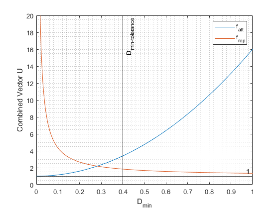
This thus yields a new vector relative to PICO’s local coordinate frame. This vector can still have a magnitude smaller or larger than 1. When the magnitude of this vector is larger than 1, it is limited to 1, such that the X and Y components of this vector can be multiplied with PICO’s maximum velocity such that the maximum velocity is never exceeded, but it still enables PICO to drive more slowly, for example when moving through a narrow corridor in which the rejective field is very strong.

During testing, it was noticed that the exit detection algorithm can sometimes rapidly switch between detected targets relative to PICO. When this rapid switching occurs, we do not want PICO to rapidly adjust its direction. Therefore when this rapid switching is detected, the vector corresponding to the gradient of the attractive field is filtered using a low-pass filter with a relatively low bandwidth. When no switching is detected, thus in the regular case, this vector is filtered using a low-pass filter with a relatively high bandwidth allowing for faster adjustment of this vector.

Of course, it is possible that at a certain time instance PICO receives a relative goal. At the next time instance it might be possible that the exit detection algorithm does not provide a goal. Therefore, each time the potential field algorithm obtains a goal, it captures the orientation of its local coordinate frame with respect to the world coordinate frame based on odometry. Furthermore, the distance to the goal relative to this local coordinate frame is logged. In the next iteration, when the potential field algorithm is called with a flag “0”, corresponding to the case that at this call, no relative goal is provided, PICO uses the odometry data to move to the last known goal with respect to the last known coordinate frame. During this motion, PICO maintains the orientation of the last known attractive field vector when a goal was still provided. Of course, when the distance to its last known coordinate frame becomes larger, the position error becomes larger. Nonetheless when the exit detection algorithm initially provides a goal which lies 1 [m] in front of PICO, and then can no longer detect this relative goal, PICO will move forward and measure the traveled distance using the odometry until it has traveled the distance of 1 [m] with respect to PICO’s local coordinate frame when a goal was provided. When this distance has been traveled, PICO stops moving. This way some additional redundancy has been built in, such that PICO can still move when no goal can be provided at a certain time instance.

Exit detection algorithm

For the Escape Room Challenge, it is not required to compute PICO's global location and orientation, i.e. its global pose, within the room. In fact, this is not even possible, because the dimensions of the room are not known and the room may also not be perfectly rectangular. Even if it were, it is unlikely that it would be possible to uniquely compute the robot pose from the LRF data. Since the mere goal of this challenge is to drive out of the room via the corridor, the exit detection algorithm must detect where the exit is relative to PICO's current position. This information then serves as an input to the potential field algorithm to compute the attractive field. Note that this algorithm, thus, serves as a means of meeting (border-)requirement 'Identify Exit'.

The following considerations are taken into account:

• Looking forward, it is decided that it is preferred to already implement as much intelligence as possible which may later function as part of the localization component of the software for the final Hospital Challenge.
• In order to feed the potential field algorithm effectively, i.e. in such a way that it is expected to yield a smooth motion, it is also preferred to first compute the center position of the start of the corridor. Only once PICO is positioned sufficiently in front of (or in) the corridor, the center position of the end of the corridor should be computed.
• Moreover, a significantly accurate estimate of these positions is required.

For this reason, instead of simply detecting gaps in the LRF data, the exit detection algorithm must be able to:

i) divide the LRF data into segments belonging to seperate walls,

ii) fit lines on these walls (to minimize the influence of LRF data noise on PICO's perception),

iii) use these fits to compute corners and edges, and

iv) use theses corners and edges to compute the target position.

The exit detection algorithm, therefore, incorporates data pre-processing, data segmentation, line fitting, corners and edges computations, and target computations. These individual parts of the algorithm will be further elaborated below.

Data pre-processing

Firstly, the LRF data is pre-processed by simply filtering out data that lies outside of the LRF range, i.e. below its smallest and above its largest measurable distances, 0.01 and 10 m, respectively. It is then converted to Cartesian coordinates relative to PICO's local frame (see Figure x):

where ρ_i is the measured distance and θ_i the corresponding angle. Note that the index i starts at 0 (and, thus, ends at 999).

Figure x: PICO's local frame and conventions.

Data segmentation

The procedure that is applied to divide the LRF data into segements is inspired by the famous image processing technique, split and merge segmentation. It is based on the criterion that, if all data points in a considered range lie within a treshold distance to a straight line connecting the first and last data point of that range, a segment is found. This approach is especially suited in the context of the two challenges, because the walls of PICO's environment are (sufficiently) straight. Moreover, the static objects of the Hospital Challenge are (sufficiently) rectangular. The iterative procedure encompasses the following steps and computations:

1. Start with the first and last data points, corresponding to θ = -2 rad and θ = 2 rad, respectively (assuming these have not been filtered out during pre-processing). Set i_{start} and i_{end}, respectively, equal to the corresponding indices (0 and 999).

2. Compute the perpendicular distances, d_i, of all other data points to a straight line from data point i_{start} to i_{end}: d_i = |(y_2 – y_1) x_i – (x_2-x_1) y_i + x_2 y_1 – y_2 x_1| / \sqrt( (y_2 – y_1)^2 + (x_2 – x_1)^2 ). Here, (x_1,y_1) and (x_2,y_2) are the Cartesian coordinates of data points i_{start} and i_{end}, respectively.

3a. Compute the maximum of all distances computed at step 2 and the corresponding index. If this distance is below a certain treshold (which accounts for measurement errors), go to step 4, otherwise, go to step 3b.

3b. Split the segment, i.e. set i_end equal to the index computed at step 3a, and go back to step 2.

4. A new segment is found. Save the indices of the first and last data point belonging to the segment, i.e. i_{start} and i_{end}. Set i_{start} to i_{end}+1 and set i_{end} back to the index of the last data point, and return to step 2.

5. Repeat this procedure until all data points are considered, i.e. until i_{start} is no longer smaller than the index corresponding to the last data point.

After the segmentation procedure has terminated, segments consisting of a number of data points that is below a certain treshold are discarded. This adds robustness, because occasionally segments only consist of 2 data points, for example, and thereby may form the 2 edges of an opening. Moreover, a sufficient number of data points is required to obtain a reliable fit.

Line fitting

Next, a line y = ax+b is fitted onto each segment by means of the linear least-squares method. It can be shown that the solution is

a = ( N_{seg}*sum(x_i*y_i) – sum(x_i)*sum(y_i) ) / ( N_{seg}*sum(x_i^2) – (sum(x_i))^2 ),

b = 1/N_{seg} * ( sum(y_i) – a*sum(x_i) ),

where N_{seg} is the number of data points in the considered segment and the sums run over index i, going from the indeces corresponding to the first data point of the segment to the last. For each segment, the coefficients a and b are stored.

A serious drawback of this approach is that it is not possible to represent vertical lines, because coefficient a goes to infinity. This means that no reliable fit is found for walls that are more or less parallel to the y-axis of PICO’s local coordinate frame. Nonetheless, it is a very simple approach that will show to suffice for exit detection purposes.

Corners and edges computations

For subsequent segments, the Euclidian distance between their neighbouring endpoints, i.e. the last data point of segment j and the first of segment j+1, is computed. If this distance is below a small treshold, a corner is assumed to be found. To compute its coordinates, the intersection of the line fits of the two segments is computed. If the distance is not below the treshold, an edge is found which is a point at which a jump in the LRF data is observed or at which there is a gap (a set of angles over which no distance within range is measured) in the LRF data. Within the context of the Escape Room challenge, the first occurs if, for instance, PICO ‘looks’ at the corridor at an angle; the latter occurs if, for instance, PICO ‘looks’ into the corridor. Edges, obviously, also occur at the first and last data point of the (pre-processed) LRF data.

For each segment, the coordinates of its first and last point are saved, whether it is a corner or an edge.

Target computations

A corridor (entrance) is possibly detected if edges occur between two subsequent segments (in order to exclude the edges at the very first and last data points). Two cases are distinguished for the situation where PICO can ‘see’ the corridor:

1. PICO scans both of the walls on either side of the corridor, i.e. PICO is located in the region directly in front of the corridor, and

2. PICO scans one of the walls of the corridor and the corner of the entrance on the other side of the corridor.

Determining which case is observed is based on the slopes (coefficient a) of the lines fitted through the subsequent segments. In case 1, the observed walls should be more or less parallel, so their slopes should be equal up to a certain treshold. In case 2, on the other hand, the walls should be more or less perpendicular, so a_j should equal -1/a_{j+1} up to a certain treshold.

In case 1, the edge that is furthest away from PICO is used. A line is drawn through it, perpendicular to the line fit of the opposite corridor wall, and its midpoint serves as target. On the other hand, in case 2, the edge closest to PICO is used. Similarly, a line is drawn through it, perpendicular to the line fit of the opposite corridor wall, and its midpoint serves as target. This method serves the purpose well, because a target is first placed at the entrance of the corridor. Only after PICO is already in front of the corridor, the target is placed further into the corridor and, eventually, at the actual end of the corridor. If the target were always placed at the end of the corridor, guided by means of the potential field algorithm, PICO will first drive on a path deemed for collision with a wall. Only when close enough to the wall, PICO would be guided along the wall, towards the corridor.

Visualization and Testing

Figure 6: Large Escape Room with an exit parallel to a wall.

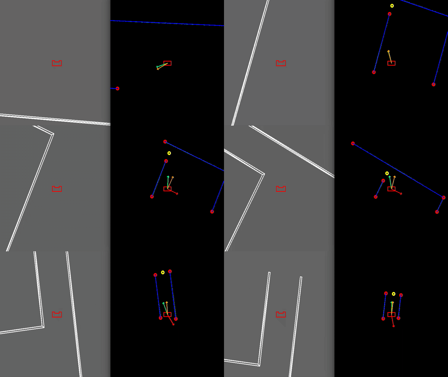
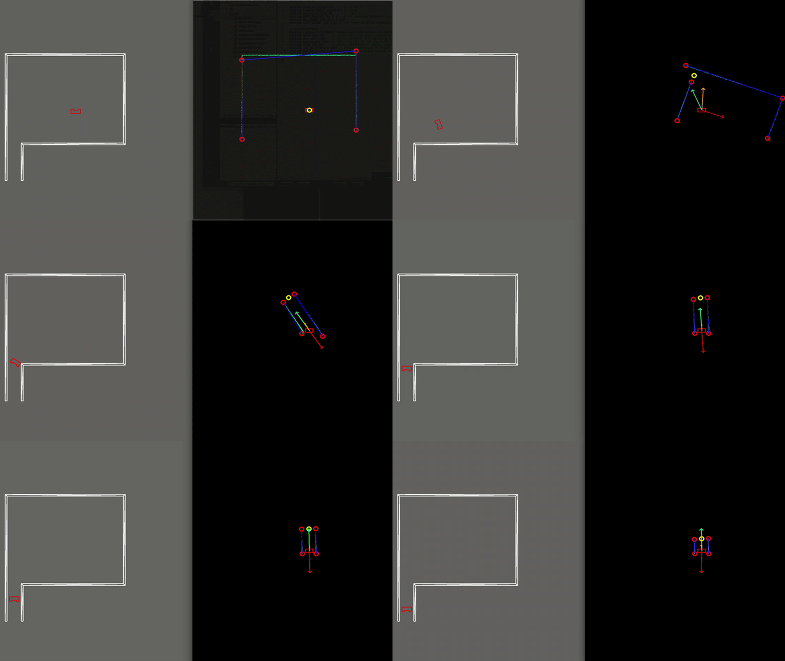
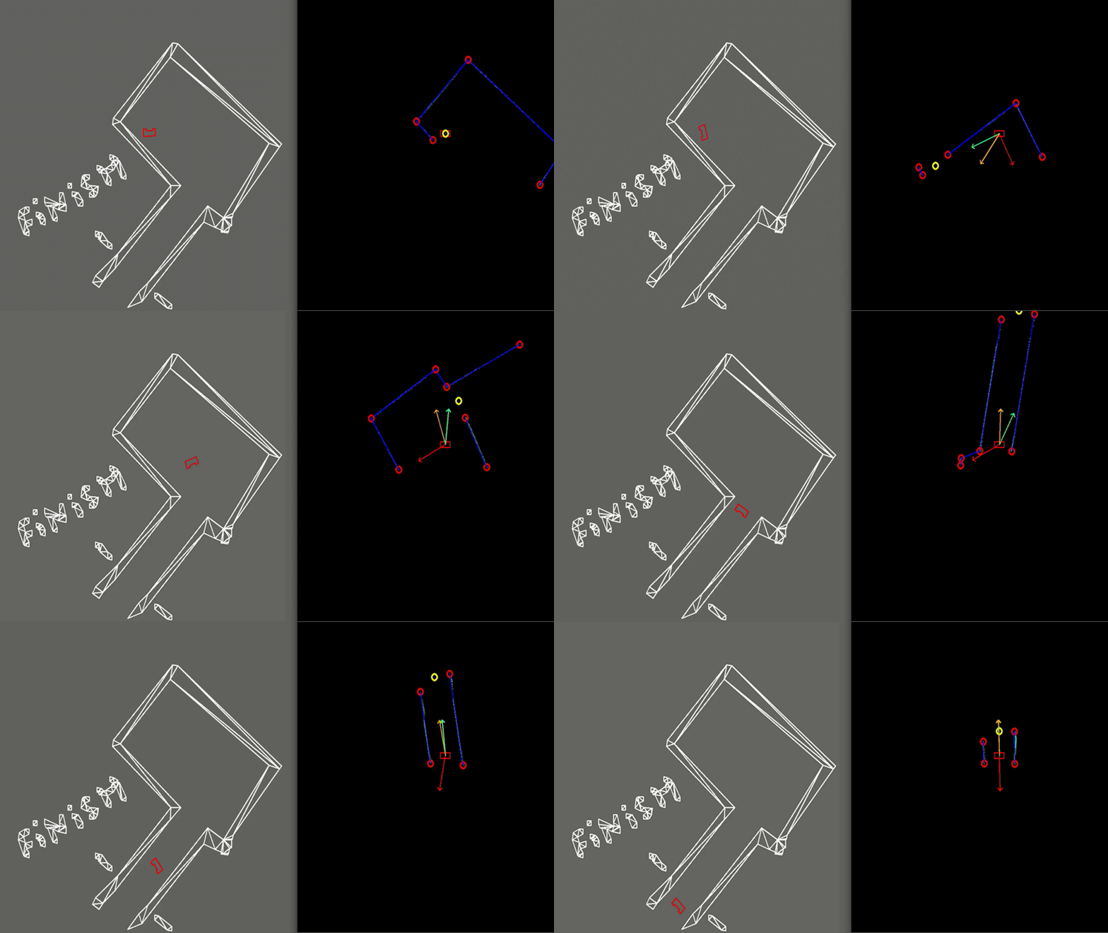
In order to see how the developed algorithm operate, a visualization is made using the openCV library. With this library dot, line, arrow, circle and rectangle shapes are created to represent the laser range data, detected walls, velocity vectors, corners and PICO respectively. These shape objects are drawn on a window iteratively representing PICO and its interpretation of the surrounding, as can be seen in figure 6.

Using this visualization, the program can be tested to optimize the behaviour of PICO. To explain main parts of the testing phase, three test cases are considered. However, a lot more cases have been tested in order to ensure robust behaviour of PICO while escaping the room.

Test 1: Large Room and Parallel Exit

As shown in figure 6, PICO is dropped in a large wide room with the exit parallel to one of the walls. In this case PICO is not able to see the whole room at ones because some walls are too far away. In this case, detection of the exit can be a challenge and therefore PICO is programmed to initially start moving away from the walls unit an exit is detected. This allows to have a better view of the room since it is moving to the center. When the exit is detected, PICO can continue to move towards the exit. In the example in figure 6, this happens quite rapidly. In case the exit would not be detectable, PICO sets a temporary target in front of him, to keep moving through the room. Detection of an exit which is parallel to one of the walls is an unique case which has been tested extensively. However, the detection algorithm had no problems to detect these special kind of exits.

Test 2: Small Exit

Another case, illustrated in figure 7, can be challenging due to the narrow exit of around 0.5 meters. Here PICO’s positioning is made accurate enough to fit through without colliding. To gain more accuracy PICO is driving slower which is caused by a larger amplitude of the rejective field in the narrow corridor, making the overall velocity vector is smaller.

Test3: Realistic Environment

As visible in figure 8, the walls of the room consist of separated blocks. The detection of the exit is made robust to these kind of gaps, by using a minimal threshold for the size of the exit. As shown, PICO does not mistake these gaps for an exit.

Figure 7: Escape Room with a small exit.

Figure 8: Escape Room with realistic wall containing gaps.

Results

Figure 9 shows the final result of the Escape Room Challenge. During this challenge, PICO managed to escape the room within 15 seconds, as fastest of all groups. In the beginning it is visible that PICO starts with rotating counter clockwise. This is done because PICO could not see the exit immediately and therefore starts scanning its surrounding. When the exit is found a target is placed, indicated by the yellow circle. Then PICO starts to move towards it, represented by the green arrow. We see that the target does not stay located at the exit, but rotates with PICO. This is because the target is updated at a lower frequency and therefore PICO remembers a fixed target relative to himself for a short period of time. When driving, PICO is pushed away from the walls by the rejective field, represented by the red arrow. The resulting velocity of PICO is represented by the orange arrow. When entering the exit, the target is relocated at the end of the corridor.

Figure 9: Final result Escape Room Challenge.

Hospital Challenge

Motivation of choices

"reason choices of algorithms based on requirement of this challenge"

Path planning

Why we need a path planner

In the Escape Room challenge a feature detection algorithm was used to find the exit of the Escape Room. This data was then used as input for the attractive field of the Potential field Algorithm, resulting in Pico having a goal (the exit corridor) to drive towards. This approach worked very well for the Escape Room Challenge, but since the Hospital Competition is much more Complex a dedicated path planner is required to guide Pico through the map and towards the cabinets.

Several options for path planning algorithms have for this cause been considered. An overview and rating of the algorithms that were examined can be seen in Table:

TOEVOEGEN

A* Algorithm

Based on the fast computation time and relative ease of implementing it was chosen to work with a grid based A* algorithm. This algorithm works as follows: In a grid of size N x M a path has to be planned from a start point towards a goal point. From the start point, all adjacent grid points that are not obstacles are evaluated, For each point n the cost g(n) is calculated to get to that node from the start node, and the cost h(n) to reach the target from that node on the cheapest path. The algorithm then goes to the node which has the lowest value for g(n) + h(n), and then starts evaluating all adjacent nodes that have not been evaluated before. Obstacles like walls have a very high value for g(n) and h(n), and are therefore aotumatically avoided by the lowest cost determination. In case a dead end is reached by the algorithm, it automaticcaly goes back to the last grid point with the lowest combined cost that is not evaluated yet. This proces is then repeated untill a path of grid points is determined from start to goal.

Creating a weighted Map

If the A* algorithm would be implemented like this, it is likely that a path would be planned directly next to walls and/or other obstacles. Since a normal grid size would be much smaller than the dimensions of Pico, it is decided to make all grid points where Pico can effectively not come also off-limit for the path planner. This is done by calculating the Euclidean distance from grid points that contain an obstacle to the grid points in its surounding. If this distance is below a certain treshold, the cost of going to these grid points becomes the same as going to a grid point containing an obstacle, therefore effectively avoiding it by the lowest cost determination. By doing so,the path is now always computed at a minimum distance from the walls.

Input for Motion Control

Several options can also be though of when it comes to tracking of the path. Smooth movement was observed when 'goal' points are used as input for an attractive field, so it is decided to use this approach again. By using a point in the path approximately 0.5m ahead of pico as input for the attractive field, and aligning Pico with the vector towards this point, smooth reference tracking is effectively achieved. Using this approach for Motion Control also makes it possible to include a repulsive field for obstacle avoidance, which will be explained later on.

A* computation time dependent on grid size -- > mention improvements

Improvements:

• Compress map for very course path planning
• (two paths, very course (complete) path and multiple fine paths) --> Lead to 'lagging' behaviour
• Only use a very course path --> lead to paths being planned through walls, squares which contain path nodes just missed walls but were planned through them
• Use a course path if possible, switch to fine path if no course path is found OR if an emergency stop has happened and an accurate path around the obstacle has to be planned

--> Show examples of typical behaviour that was observed and elaborate choice of last option

Elaborate on Recovery state

Deliverables

Design Document

In the design document, a generic approach for the Escape Room Competition and the Hospital Competition is introduced. Requirements are proposed, which are clarified by means of specifications. Based on these, a finite state machine is designed. In each state, groups of functions are proposed. This functionality is, in turn, structured in an information architecture which covers the components and the interfaces. Undoubtedly, throughout the remainder of the course, this document needs to be updated, but its current content functions more as a guideline. Since the Escape Room Competition is the first challenge, functional specifics may be more focused towards this goal. And because software design is use-case dependent, for the Hospital competition the current approach will need to be adapted and improved. The design document deliverable can be found here.