Embedded Motion Control 2019 Group 9

Group members

Nicole Huizing | 0859610
Janick Janssen | 0756364
Merijn Veerbeek | 0865670

Design Documents

The Initial Design document can be found here: File:Initial Design Group9.pdf

The powerpoint presentation about the design is in this file: File:Presentation initial design.pdf

The powerpoint presentation about the final design can be found here: File:Presentation final design group9.pdf

Logbook

The composition of group 9 has changed twice. At first, George Maleas decided to quit the course at the 13th of May, two days before the escape room competition. At second, Merijn Floren also quit the course on the 3rd of June. The motive for both students was that they lacked the c++ programming skills to meaningfully contribute to the project. Participating in the course would take a too large investment of their time. The code for the final challenge was written by Janick Janssen, Merijn Veerbeek and Nicole Huizing.

Code

Link to code for aStar path planning: https://gitlab.tue.nl/EMC2019/group9/snippets/132

Initial design

<<Mostly based on hospital challenge. Some remarks for escape room challenge can be made.>>

Requirements and specifications

Requirements	Specifications
Operate autonomously	Read in prior given map Obtain data through LRF and odometry, operate with SLAM and path finder
Visit cabinets in order given at challenge	Executable takes in desired cabinet order
Indicate task progress	"Speak" on arrival at cabinet Take snapshot of cabinet
Avoid deadlocks (30 seconds) or infinite executions	Have PICO recognize these situations and return to an earlier/random point before continuing to the task
Obey speed limit	Ensure rotational speed is limited to 1.2 rad/s, translational velocity to 0.5 m/s
Finish within 10 minutes	Limit the computational expense of the code Ensure smooth movement
Prevent collision	Keep a safe distance from walls and objects
Proper termination	Stop after having performed interactions at the final cabinet
Additionally, identify (moving) objects	Track unexpected points, add to map for statics temporarily for moving

For the escaperoom challenge these already held too, with the exceptions that PICO should properly stop after the finish line and that the task should be completed within 5 minutes.

Functions

Janick, probably handy to have a cleaned up code first

Components

Janick Hardware as initially given (LRF+odometry, actuators, computer, pico dimensions a x b)

Interfaces

Merijn

Escape room challenge

For this assignment, we decided to work out two different strategies. The first one is the wall following strategy and the second one is the direct exit detection strategy. The idea was that the detection, drive control and world model code could be shared between both strategies and that only the planning module would be different. Pico should first try to use the direct exit detection strategy. If he fails to find the exit, Pico should change to wall following strategy. Since the direct exit detection code was not yet robust enough during the escape room competition, the code that was used in the challenge uses only the wall following module.

The table below presents an overview of the most important functionalities that Pico should have to compete in the Escape room competition.

Wall following	Direct exit detection	Both
Rotate until aligned to right wall	Detect convex corners when seeing both walls	Walk through the hallway
Walk while staying aligned to right wall	Detect convex corner when seeing only one wall	Cope with wall misalignment
Detect exit from laser data on right side	Rotate and move to exit entrance point	Stop after reaching exit
Rotate to exit entrance		Prevent bumps at all times
		Cope with odometry deviations caused by slip

Code architecture

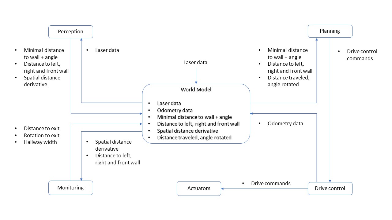
In the figure below you can find a schematic representation of the code architecture that we used:

Interfaces

World Model

The class 'WorldModel' functions as main storage place for important variables that can be used by all other modules. To enhance separation of tasks among the different modules, all values stored in the World Model are private. The class also has some public functions by which other modules can obtain and process data.

The most important variables in the World Model will be explained here. The first one is the minimum distance to a wall, accompanied by the angle where it is found, relative to Pico. These values are used to allign Pico to the right wall and turn left in a corner. When the shortest distance to a wall is found on the right of Pico, he can walk straight ahead. However, if the angle is outside the margins, Pico will rotate either clockwise or anticlockwise until he is aligned to the wall again. If the shortest distance is found in front of pico, he will turn left until the closest wall is found on the right again.

The other important data structure in the World Model is a matrix, in which the spatial derivatives are saved. By spatial derivative, we mean the difference between the measured laser distance of one array and the next evaluated array. Between these two arrays, 4 arrays are skipped.

Detection

closest convex corner detection

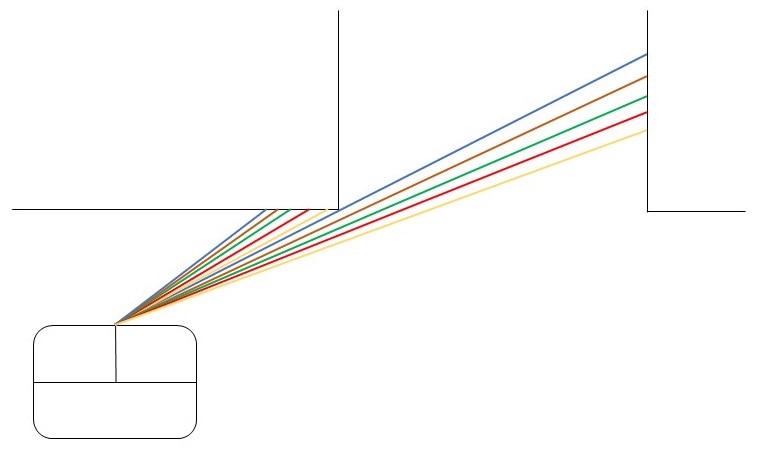
The laser data is called in the World Model and sent to the class 'Perception'. In this class, the laser data is converted to important variables as the minimal distance to a wall, the accompanying angle relative to Pico and the spatial derivative matrix. These values are then updated in the World Model.

In the class 'Monitoring', the output of the class 'Perception' is converted to useful information about the exit. There are two ways of detecting the exit. It depends on Pico's initial position which way should be used. If Pico is standing within the area extended from the two corners of the exit, Pico will see both walls of each convex corner. If Pico is located outside this area, it will only perceive one wall belonging to the closest convex corner and both walls of the furthest convex corner. For both situations, the matrix with spatial derivatives can be used.

First, there will be sought for a "gap" in the spatial derivative data. If the difference between the laser distance of one array and the array 4 steps further is above a certain threshold value, the angle of the first array is saved. This evaluation will be done for all arrays. By leaving 4 arrays in between, a real convex corner will have a higher occurrence than a small slit in the wall. A cluster of laser arrays with a high occurrence is expected to be the closest convex corner. In the figure on the right, the color combinations of laser arrays will give a high spatial difference. This cluster of arrays will be recognized as a convex corner.

Next, the spatial derivative matrix will be scanned for transitions from negative derivatives to positive derivatives. In this way, the furthest convex corner can be found (or both convex corners if Pico is between the corners).

The sideways, forward and rotational motions Pico needs to make to get to the entrance of the hallway are calculated. These values are stored in the World Model.

Planning

The global planning is defined in- and executed by the main program. To this end, a finite state machine is used. Pico starts by initializing all classes and sensors. If Pico is too close to a wall, he drives away from it. Next, it enters the 'direct exit finding' planning. It tries to localize an exit from its current position. If Pico fails to find an exit, he will turn around 180 degrees and try again. In this way, Pico should have observed every angle of the room. If Pico finds the exit, it will move toward the entrance, following the drive commands that were determined in the 'Monitoring' module. To account for slip, this procedure of localizing the exit and driving towards it will be repeated until Pico is close enough to the hallway entrance point. Now, Pico drives straight ahead and enters the state 'hallwayFollow'. In this state, Pico drives forward if it is not too close to a wall on both sides. He moves right if he is too close to a wall on the left side and moves left if he is too close to a wall on the right side. This procedure continues until Pico does not perceive a wall on the left and right side anymore. Pico stops and shuts down the program.

If still no exit is found after rotating, Pico switches to the 'Wall following' planning. Pico walks straight ahead until it finds a wall. He turns left until he is aligned to the wall and follows the walls, driving counterclockwise to the exit. If a large transition of the laser distance on the right of Pico occurs, Pico turns clockwise and moves sideways until it is standing in front of the hallway. Now Pico drives forward and enters the state 'hallwayFollow', which it only leaves when no walls on the side are detected and Pico has crossed the finish line.

Controller

The module 'driveControl' consists of a collection of functions. These functions are driveForward, driveBackwards, driveLeft, driveRight, rotateLeft, rotateRight and stop. Rotational and translational speed are fixed values that are stored in a configuration file. Each function updates the odometry data to keep track of the drive effort.

Wall follower

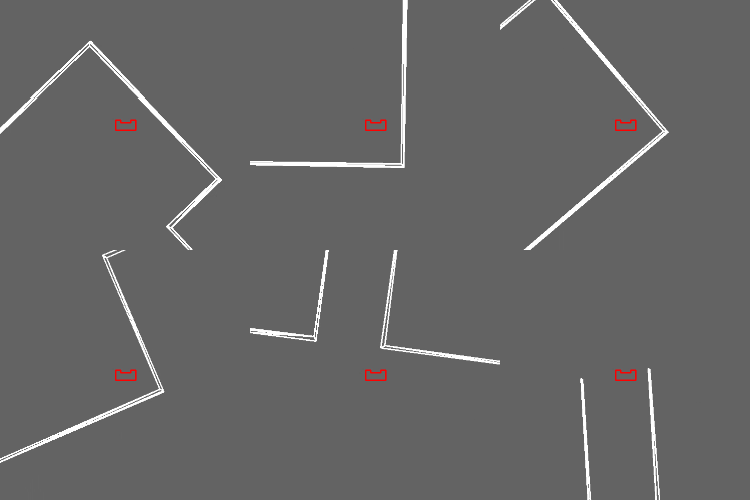
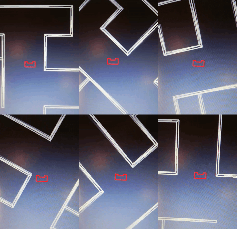
In the movie on the left, one can see a simulation where only the wall following strategy is used. As you can see in the movie, Pico walks to the wall and enters the wall-following module in which it adjusts itself when its angle with the right wall exceeds a threshold value. When he detects the gap at the right side, it turns towards the exit and enters the hallwayFollow module.

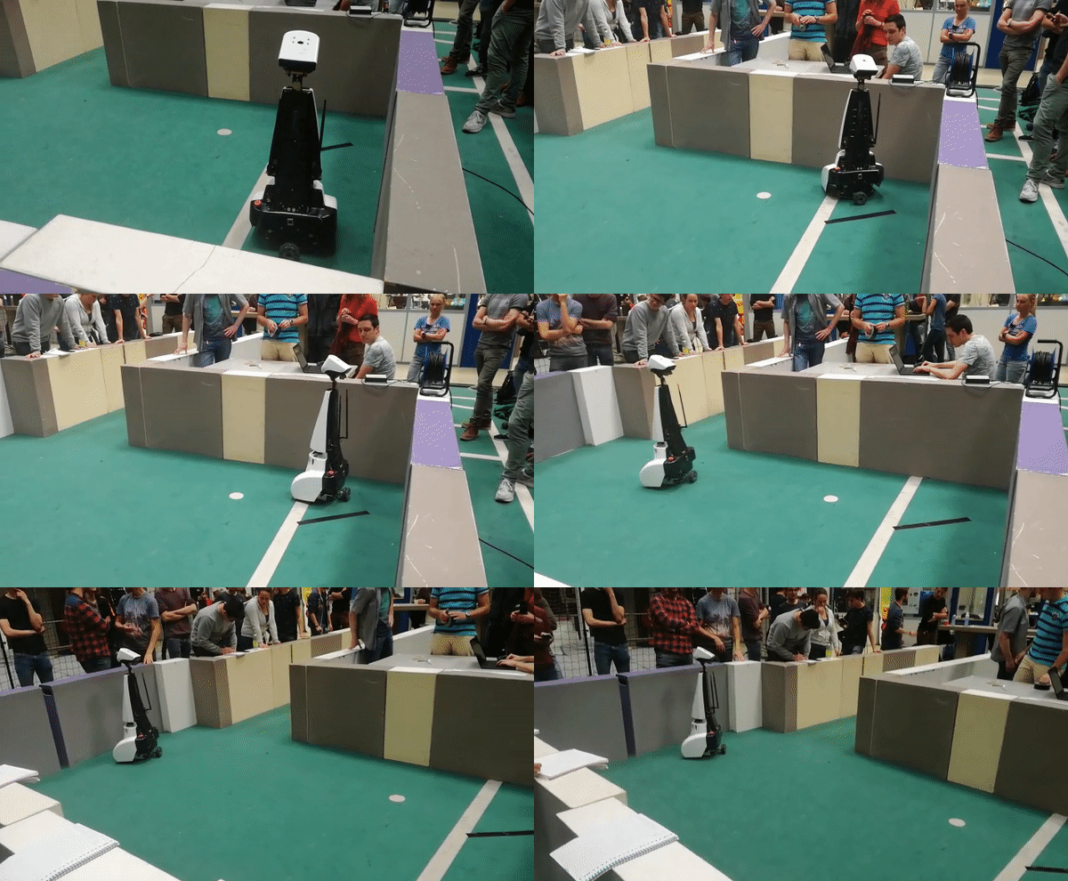
In the movie on the right, the real test-results are shown. The behavior of Pico differs from the simulated situation in two facets. At first, Pico tends to rotate too far, building up an angle with the right wall. It does not rotate to compensate for this. This lack of reaction is caused by choosing too high safety margins. At second, Pico does not turn towards the exit. Later, we found out that this was due to a missing absolute value in the calculation of the difference between laser range values on the right side of Pico. In the simulation, the gap on the right side gives very low laser range values, while in reality the gap gives relatively high laser range values with respect to the wall Pico is following. By taking the absolute value, this problem would have been addressed.

Simulation performance

Escape room challenge performance

Reflection

Both previously mentioned points could have been remedied if we would have used the test sessions more efficiently. The full code was not finished yet when we had the last test session before the challenge. We could better have focused on either the wall following strategy or the direct exit finding strategy. By choosing to do both, we got our self into time problems.

The code itself features all modules that the code should have. However, in the communication between the modules, some improvements can be made. The code would have been more readable if we would have used flags to control the state of the state machine. Now we send a lot of data from the world model to the state machine to assess whether a state should be left and a new state should be entered. Also, we could have sent the state of the state machine to the world model and connect with the drive control from the world model. At last, the code for exit detection was written too much in a sense-plan-act manner. This method is prone to failure, especially when data is inaccurate.

Exitfinder

explanation & movie of simulation (do we have something useful?) & discussion on approach - Janick

Alternative check for big jumps corners at derivative switch comparison point by point, work, but... → not robust slits in the wall break method even with averaging, (potentially due to not handling rp’s) get old code back from git or use old phone vid

exitescape

Hospital challenge

World model

Merijn

Perception

Janicks

Also simulation movie of updating map possible?

Read in data. (throwaway endpoints → observed to be line, but time constraints) identify rupture points (veryfarawaypoints) identify bps (adaptive breakpoint adapter [j1]) throw away lonelys; unreliable /image:lonelies identify suspected corners (have to be convex), make initial line segmenu detect corners (IEPF,[j1])

corner type identification check number of subsequent segments → curved object → suspected dynamic \video green linepieces, red bp’s, orange rp’s, blue circles convex, purple concave, cyan assumed (convex), yellow/or gray maybe lidar simulated data reference points, text added in afterwards

Mapping Points of interest (generalised corners and linesegments) Through localisation → map frame points of interest/walls stored. Compare new data with known and expected. New cornerpoints are added with a timestamp, if this fluctuates heavily they're removed, otherwise we see a static object. PICO should stop when observing new point. To prevent stopping continuously these are only the generalised corners, or a new linepiece, points related to said linepiece are allowed to be added “on the run”. Also simulation movie of updating map possible? Tbd, i’m going to check to open/close/open adjusted maps, if internal state is conserved this should allow for display of object detection functionality. [j1] Borges, G.A.; Aldon, M.J. Line extraction in 2D range images for mobile robotics.J. Intell. Robot. Syst.2004,40, 267–297. [CrossRef]

Localization

In order to know in what direction PICO should go, it needs to know its current location. To achieve this, PICO has been given a localization module. This module makes use of Monte Carlo localization (MCL). The module tries to determine the location of PICO on a pre-known map of the surroundings. The current location is used to determine the path to the next destination and to make PICO follow that path.

The map the world isdivided into several grid points. The goal of the localization module is to determine on which gridpoint PICO is and with what orientation. It is not required to know the exact grid point, because the grid points are used for the global movement of PICO. To move PICO more precisely, for example when it needs to allign to a cabinet, PICO does not make use of the current grid point, but it alligns itself by the laser data.

The current grid point of PICO is determined in the following way. The initial starting area of the Hospital challenge is roughly known. This information is used to reduce the possible locations of PICO. The gridpoint in the middle of initial starting area is chosen to start the MCL. All grid points within a certain distance of this gridpoint is added to a list. The gridpoints in this list cover all possible starting positions in the initial staring area. Multiple particles are created for each grid point in the list, each with a different orientation. The MCL module must try to find which particle has the most likely location and orientation of PICO.

When PICO has moved, the current location can be estimated based on the old known location and the odometry data. This gives a starting grid point and orientation to create the particles. Because the rough orientation is known, the number of particles can be reduced, because the likelyness of certain grid points and orientations are very low. For example, if it is known that PICO is facing north and it has turned about 5 degrees according to the odometry, it has no use evaluating particles facing south. It is only required to check particles which have an orientation of 5 degrees of the north, but a larger range is used to make sure that the particles with the correct location and orientation is in the list of particles.

The image below is a small example of how the particles are created. In this example, there are 9 grid points. Each grid point has different 5 orientations. That means that there are 45 particles in this example. The real implementation uses a grid of 1 squared meter with grid points space 10 cm apart from eachother. The orientation of the particles have a range between 45 degrees clockwise and 45 degrees anticlockwise of the orientation of PICO, with a stepsize of 1 degree.

Path planning

Nicole

Global path planning

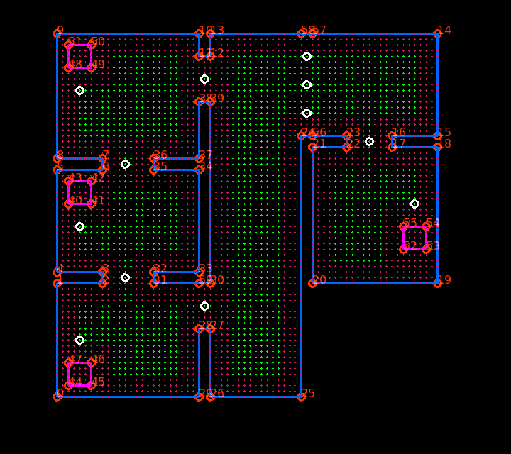
The hospital is divided in structs 'room'. This is done both to preserve the semantics and for practical purposes: it reduces computation time for local path planning and it makes it easy to call information about corners and cabinets in the proximity of Pico. A 'door' is a separate struct. The connections between all rooms and doors are stored in a graph. A vector 'globalPath' is filled by repeatedly choosing the connected door/room with the highest ID-number (if there are more possibilities). ID's that are already in the path are ignored to prevent Pico from walking in a loop. When a doorway is blocked, the connection will be removed from the graph. The route calculated in this way is not per definition the fastest route, but this is not needed to succeed in the challenge.

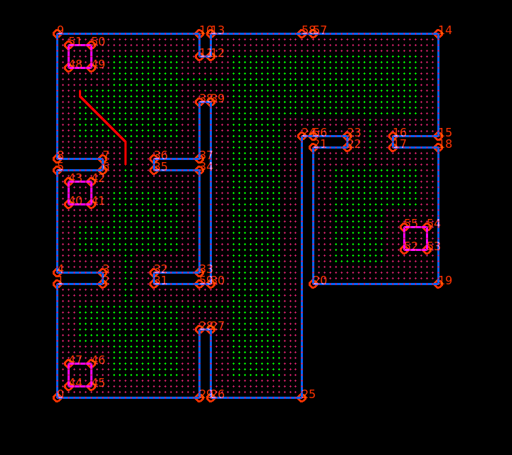
Each cabinet and each door have a unique enter-gridpoint. These points are used for local path planning. As the "large door" connecting the two parts of the hallway could be partly obstructed, three enterpoints are assigned to this door. If no obstruction is present, the middle node will be used. The enterpoints can be viewed as white circles in the image left below.

Local path planning

To plan Pico's path between enter-gridpoints, use is made of an A* pathplanning algorithm. This method was chosen over Dijkstra's method because it is faster. We will choose a heuristic function that is admissible, so it will be guarenteed that A* will give the shortest path from start to end.

All grid points on the map come with a boolean "accessible". Points that are close to a wall or an object receive the value 'false'. Mapping new objects is also based on this principle: whenever a new static object is detected, the gridpoints it covers will become unaccessible.

After the A* function is called with a certain start-gridpoint and end-gridpoint, it first goes through some checks. These checks assess whether the startposition and endposition are accessible and whether the startposition is the destination itself. If the startposition is unaccessible, the gridpoint itself and the points directly around it are temporarily made accessible (this is needed when Pico accidentally got too close to a wall or object).

Next, the start-node is put in the open list. At every cycle of the loop, the node in open list with the smallest f-value is evaluated. The f-value of node n is the sum of the cost of the path from start to node n and the heuristic cost of that node. This current node is put in the closed list. Next, the eight nodes around it are evaluated. If one of the nodes is the destination, the path from start-node to destination-node is reconstructed. If not, the cost-functions of these nodes are updated and if they are not yet in the closed list, they will be added to the open list from which the node with the lowest f-value will be evaluated in the next loop.

Grid map with door- and cabinet-enterpoints

Grid map with A* route

Finite state machine

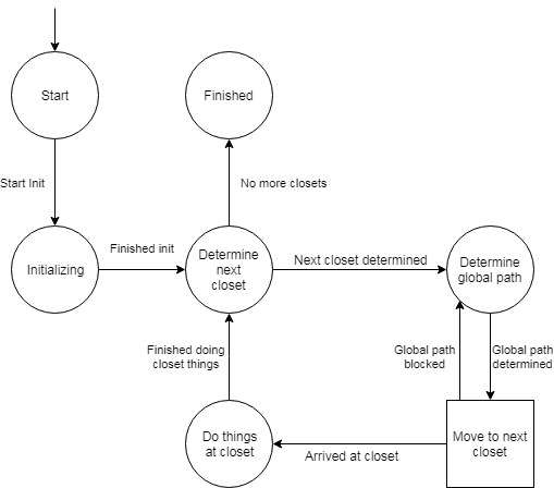
To determine which actions PICO should execute, a finite state machine (FSM) is implemented. The finite state machine is divided into 2 part: the main FSM and the drive FSM. The drive FSM is actually a sub-part of the main FSM, but it is split for a better overview and easier maintenance of the code.

The main FSM controls the global planning of PICO. The initial state of the main FSM is the initialization state. In this state, the world model and all other modules, like the perception module, are initiated. The json file is read and from this data a map of the world is constructed. The localization module determines the initial position and orientation. Once everything is initialized, the FSM switches to the next state. In this state the next cabinet that has to be visited will be determined. This cabinet object will be stored in the worldmodel. Once the next cabinet is determined and set, the FSM switches to the path planning module. In this state, it will determine which rooms PICO has to visit and in what order. This global path is saved to the worldmodel. When the global path is determined, the FSM will switch to the driving state, which is described in more detail below. Once PICO arrives at the cabinet, it switches to the next state. In this state PICO will take a snapshot of the laser data and saves the snapshot. Then it will switch back to the state in which it determined the next cabinet and the loop starts again. If PICO has handled all cabinets, it will switch to the finish state and can be shut down.

Main finite state machine

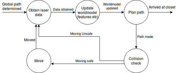
When PICO has determined the next destination, the main FSM switches to the driving state. In the driving state, the states of the drive FSM are "activated". (The main FSM actually switches to the "initial" state of the drive FSM) The drive FSM is a continuous loop of different processes. The first process in the loop is obtaining laser data. After the data is obtained, the worldmodel is updated. The perception module takes the laser data and updates the map and various other variables and saves them to the worldmodel. Once the worldmodel is updated, PICO switches to a new state. In this state, PICO first determines if the destination is reached, based on the updated worldmodel. If this is the case, the drive FSM will be "disabled" by the main FSM switching to the next state. If the destination is not reached yet PICO will determine the local path to the next destination of the global path. First PICO evaluates if the old planned path is still viable. If this is the case, it will continue following that path. This will save compuation time. If the old path is not vialbe anymore PICO will calculate a new path. With a viable path is available, PICO first does an additional check to check if the next move action is safe. The additional check is added because an object could have moved on the new path during the path calculation since the last time PICO obtained laser data, although this situation is very unlikely because time between obtaining the laser data and finishing the recalculation of the path is small) If the path is safe, PICO will move a step and then it will start the loop again. If the path is not safe, PICO will not move and will start the loop again.

The drive FSM will first try to find a path to the next destination of the global path. If it is not possible to create a path, because the path is blocked by a closed door for example, the main FSM will switch back to the global path planning state. Then it will create a new global path while not using the blocked points.

Drive finite state machine

Results

Nicole

The video below shows the performance of Pico in the final challenge. We have to say that this is not exactly the result we hoped for. As can be seen, Pico has difficulties finding the entrance of the first room. This problem is due to an unfixed bug in Pico's localization. Pico manages to determine it's global route to cabinet 0. He starts it's local route to it's first destination: the doorway of the first room. However, he turns a bit too far and heads to the corner of the doorway. Pico is programmed to step back when he is too close to a wall. After reaching a certain backward distance, Pico relocalizes itself and recalculates a path to it's destination. However, due to the problem in localization, he thinks he is outside the zone where he expects himself to be. He now re-takes the old route until he gets too close to the wall again and stays in this loop forever.

Hospital challenge performance

Discussion

Janick