Mobile Robot Control 2020 Group 4: Difference between revisions
| Line 190: | Line 190: | ||
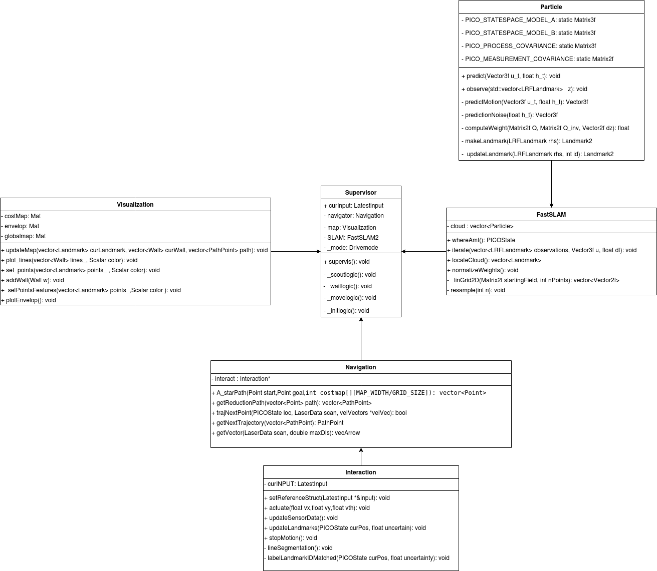
The sub-classes that are directly underneath Superivsory are Navigation, FastSLAM, and Visualization. The abovementioned algorithms are divided into these sub-classes. The Navigation contains the A* global path planning, velocity vector based movement, a local potential field, and feature detection. The Navigation class has a sub-class named Interaction, which is the only connection point to the PICO robot. The reading of the sensors and the control of the movement takes place in this class. However, since these readings are needed in other classes a struct is made, which contains all the useful information based on the current readings. This struct is made in the supervisor class and is linked to the address of a similar struct in the Interaction class. The current readings and detected features are now available in the supervisor class and can be from there. The FastSLAM class is a class fully based on the FastSLAM algorithm with a sub-class Particle which plays an important part in the algorithm. The Visualization class is based on the visualization and maintaining the map of the environment. | The sub-classes that are directly underneath Superivsory are Navigation, FastSLAM, and Visualization. The abovementioned algorithms are divided into these sub-classes. The Navigation contains the A* global path planning, velocity vector based movement, a local potential field, and feature detection. The Navigation class has a sub-class named Interaction, which is the only connection point to the PICO robot. The reading of the sensors and the control of the movement takes place in this class. However, since these readings are needed in other classes a struct is made, which contains all the useful information based on the current readings. This struct is made in the supervisor class and is linked to the address of a similar struct in the Interaction class. The current readings and detected features are now available in the supervisor class and can be from there. The FastSLAM class is a class fully based on the FastSLAM algorithm with a sub-class Particle which plays an important part in the algorithm. The Visualization class is based on the visualization and maintaining the map of the environment. | ||
Due to the iterative process nature of a robot | Due to the iterative process nature of a robot, the software is also designed on this bases. Every iteration starts with sensor reading and pre-processing of this data. The sensor data consists of laser and odometry data. The pre-processings part, processes the raw sensor data in such a way that it is usable for the next processing part. The data is now usable for the main step in the iterative process, the so-called processing step. The pre-processed data is the basis for the different algorithms, that are run in this part of the process. The outcome of the different algorithms are stored and are available in the next iteration. | ||
=====Course Paradigms===== | =====Course Paradigms===== | ||
Revision as of 11:03, 23 June 2020
Mobile Robot Control 2020 Group 4
Group Members
| Name | Student Number | |
|---|---|---|
| M. Katzmann | 1396846 | m.katzmann@student.tue.nl |
| B. Kool | 1387391 | b.kool2@student.tue.nl |
| R.O.B. Stiemsma | 0852884 | r.o.b.stiemsma@student.tue.nl |
| A.S.H. Vinjarapu | 1502859 | a.s.h.vinjarapu@student.tue.nl |
| D. van Boven | 0780958 | d.v.boven@student.tue.nl |
| R. Konings | 1394819 | r.konings@student.tue.nl |
Introduction
Welcome to the wiki page of group 4 of the 2020 Course Mobile Robot Control. The goal of this course is to design and implement software to the PICO robot which allows it to complete two different challenges, the escape room challenge, and the hospital challenge. Both challenges are in a simulated environment and should be successfully completed by the PICO robot autonomously. A design document is delivered before participating in these challenges which describe the overall architecture of the software.
Design document
The design document describes the architecture of the software. The document is divided into the requirements, functions, components, interfaces, and specifications and is relevant for both the escape room challenge and hospital challenge. However, the document should be considered a guidance for both challenges, and the initially declared functions and software architecture are subject to change as the project progresses.
Escape room challenge
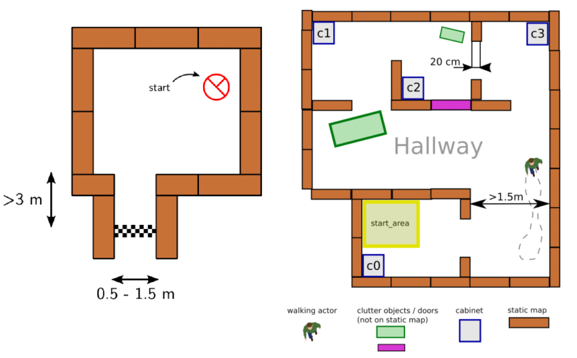
This challenge is designed as an intermediate challenge. The goal of the escape room challenge is to have PICO escape a rectangular room by exiting this said room through a corridor as fast as possible. The dimensions of this room are unknown as well as the initial position and rotation of the PICO robot. The corners of the room are not perpendicular but vary around 90 degrees. A simple example map of the room is provided before the challenge, which can be seen in figure 1. During the escape of the PICO robot, walls, static and dynamical objects may not be touched, but slightly touching is allowed.
Hospital challenge
The goal of the hospital challenge is to have PICO autonomously maneuver through a simulated hospital environment. The hospital environment consists of multiple rooms and a hallway. Each room contains cabinets and the objective is for PICO to deliver medicine from one cabinet to another, where the order will be defined by the judges beforehand. Similar to the escape room challenge, the dimensions of the map and the initial position and rotation of the PICO are unknown. However, the starting room will be provided beforehand. During the delivery of medicine by PICO, a handful of static and dynamical objects will be in PICO's way. It is PICO's job to avoid collision with any objects or walls and deliver the medicine in the correct order as fast as possible. An example map of the hospital environment is provided, which can be seen in figure 1.
Design Document
This document describes the design of a PICO application. There are two competitions for the robot to complete. The escape room competition, where the robot needs to escape out of a rectangular room, without bumping into a wall. And the robot needs to complete the hospital competition, where the robot needs to maneuver through a hospital, where it has to avoid obstacles. This document should be considered a guidance for both challenges, and the initially declared functions and software architecture are subject to change as the project progresses.
Requirements

A requirement tree is constructed with the requirements of the stakeholders of the project. The stakeholders are the customer, the hospital employees, and the developers of the robot. From here on, the environmental requirements, indicated with the orange boxes, have been acquired. From these environmental requirements, the border requirements, indicated with the purple boxes, have been acquired. Lastly, the system requirements have been acquired, indicated with the green boxes. Some of the green boxes have a set value assigned, indicated with a blue ball. And other system requirements are out of scope for the project team, indicated with a red square. The requirement tree of the hospital challenge can be seen in figure 2. The requirement tree of the escape room is indicated with the red dotted line.
The values assigned to system requirements are still subject to change as the project progresses. In addition, two values have not been chosen yet. Namely the maximum acceleration and the maximum distance to walls and objects. The maximum acceleration will be chosen accordingly once more information about the robot is available. The maximum distance to walls and objects has been chosen between a range from 0.1 and 0.5 meter and will also be chosen accordingly later on when more information is available.
Functions
In this section, the proposed architecture is described by means of its constituent functions and their relationships (interfaces) between one another.
PICO interfaces
These are all low-level interactions consisting mostly of calls to the IO API (which represents communication with PICO).
- Actuate(v, u, th): Casts a desired velocity profile [x′, y,theta″] to the robot.
- getLRF(): Pulls LRF data from the robot. Returns a laserdata struct.
- getODO(): Pulls odometry data from the robot. Returns an OdometryData struct.
Mapping
This section describes the outlines of the internal map model and its learning process.
- seeLocal(Laserdata): Interprets laser data as a local vision envelope, and stores the outcome locally.
- loc2glob(): Transforms local sensor data into a global perspective using calibration elements (e.g. intersections of wall lines).
- tf2map(): Transforms sensor data (in a global coordinate system) to Mapdata, which involves rasterizing the received data.
- integrate(): Compares and contrasts new data with old data, and modifies (and/or expands) the global map model accordingly.
This section covers the system functionalities responsible for (intelligent) navigation. All functions here have read access to the world model’s internal map and LRF envelope.
- localize(): Deducts the PICO’s current location in the map model based on its most recent LRF data.
- pathfind(x, y): Employs a pathfinding algorithm to find a combination of rotations and straight motions (longitudinal or sideways) that will bring the PICO from its current location to the global coordinate (x, y). Returns a PathData struct that describes the intended locations, and necessary rotations and local (x, y) motions to reach them.
- nextTrajectory(): Takes the next first data from PathData, and calculates the necessary velocity profiles and timings to achieve the desired motion smoothly. Returns this as a Trajectory struct.
- compensate(): Checks the PICO’s current location compared to its intended location within the planned path and determines whether compensation is needed in the sense of adjusting the path, the PICO’s position, or recomputing the path.
Supervisor
This section covers the governing control logic of the proposed system. The idea is that the supervisor makes choices, tunes parameters, and controls flow-of-command within remaining code depending on its mode and changes modes dynamically. Modes are described here as functions but may end up in a different form during implementation.
- init(): Initializes the robot, checks (as far as possible) whether safe operation is possible. Sets the mode to scout.
- scout(): PICO is uncertain about its surroundings, and hence scans its surroundings, moving as little as possible in doing so. In this mode, safety parameters are conservative. Once a useful feature (such as a door) is found, or map confidence improves enough for PICO to feel safe, control is yielded to the move mode. If all exploration options are exhausted and PICO is still uncertain, control is instead yielded to wait.
- move(): PICO knows enough, and knows where it wants to go. This mode sets safety margins much more aggressively than scout mode and looks to move long, efficient motions in pursuit of PICO’s intended destination. During motion, PICO keeps updating its map, and reverts to scout mode if certainty dips to unacceptable levels.
- wait(): PICO decides its goal is currently impossible. Waits, and occasionally returns to scout mode to see if the situation has changed.
- act(): An empty token mode to represent PICO arriving at a destination and doing something there.
Interfaces
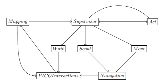
Keeping the aforementioned functionalities in mind, and given that the modes of the Supervisor module are represented here as separate locations for clarity’s sake, a rough depiction of the proposed system structure is shown in Figure 3.
Components
The hardware of the PICO robot used to smoothly execute the functions mentioned above, consists of the following components:
- Sensors
- Laser Range Finder
- Wheel encoders
- Actuators
- Holonomic wheels
- Computer
- IntelCore i7 Processor 8+ GB of DDR3 RAM
Specifications
System: PICO
- Maximum translational velocity: 0.5 m/s
- Maximum rotational velocity: 1.2 rad/s
- Wheel encoders used for odometry
- Laser Range Finder used for distance measurement
- Measurable angle: 4 radians
- Resolution: 0.004 radians
Environment
- Escape room challenge
- Shape of the room is rectangular
- PICO starts at a random position
- Width of the corridor is between 0.5m to 1.5m
- Finish line is more than 3m into the corridor whose orientation is perpendicular to the wall
- Walls are not necessarily perfectly straight
- Corners are not necessarily perfectly perpendicular
- Challenge is to be finished within 5 mins
- Hospital challenge
- Hallway is approximately 1.5m wide and is not necessarily straight
- Doors in the hospital are 0.5m to 1m wide. (closed or open)
- A random number of static and dynamic obstacles will be present throughout the hospital
- Challenge is to be finished in 5 mins
Escape Room Challenge
To safely get the PICO robot to the exit of the escape room, the strategy to implement a wall-follow algorithm is chosen. If the Algorithm is implemented successfully, it should be a safe and quick solution to the problem. The PICO will move to a wall, after which he will align perpendicular to the wall. When aligned to the wall, PICO will move left until it reaches either a wall or a gap. It will choose to rotate or drive into the gap accordingly. This algorithm was chosen because it is a reliable algorithm that, if implemented successfully, is a relatively quick escape.
Software architecture and implementation
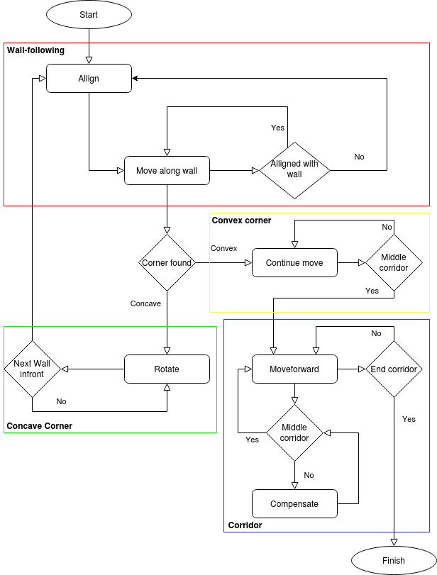
The wall-follow algorithm is divided into the following sub-parts:
Step 1: The PICO moves forward
- The PICO moves forward until it reaches a wall. The PICO will start at a random location inside the escape room. This means the robot can be anywhere inside the room. Thus, the first thing PICO does is move forward until it detects a wall getting closer. As the wall gets closer, the velocity of PICO decreases until it reaches a certain threshold from the wall, which means the PICO will stop moving.
- Implementation
- For this step, a simple function called goToWall(alignDistance) is constructed. This function lets PICO move forward while continuously checking if the minimum distance from PICO to any surrounding wall is smaller or equal to the given alignDistance threshold. If this is the case, the movement for the PICO stops and step 2 will be initiated. The closer PICO comes to any surrounding wall, the lower its velocity will become.
Step 2: The PICO aligns to the wall
- When PICO reaches the wall and completely stops moving, PICO starts rotating. It will rotate until it is perpendicular to the wall. This is achieved by having PICO stop rotating once the middle LFR sensor has the smallest value. Here, the rotational velocity also decreases when the distance to the endpoint decreases.
- Implementation
- To align PICO to the wall as accurately as possible, the function alignWall(vx, vy, distWall) is constructed. Here, the rotation difference between the wall and the PICO is used to adjust the rotation speed of the PICO. The closer PICO is to the end goal, thus the rotational difference is getting smaller, the smaller the rotation speed is until it reaches the end-goal of being aligned perpendicular to the wall. After reaching perpendicularity, PICO continues with step 3.
Step 3: The PICO follows the wall
- Once the PICO is perpendicular to the wall, it is ready to start following the wall. This is done by moving the PICO to the left until it detects a corner. If the PICO detects a convex corner, this means there is a corner approaching, and if the PICO detects a concave corner, this means there is a corridor approaching. The PICO will align to the new wall and repeat step 3 when there is a corner detected and it moves to step 4 if a corridor is detected.
- Implementation
- The function followWallTillNextWall() is constructed in such a way that PICO will go left after it is aligned to a wall. The function continuously checks if there is either a convex or concave wall approaching from the left. In case PICO detects a convex wall, it will use the function rotateTillNextWall(angle) until it is perpendicular to the new left wall and repeat step 3. In the case of a concave PICO continues to step 4.
Step 4: The PICO detects corridor
- The PICO drives a little further until the PICO is aligned to the exit. Once it is aligned to the corridor and feels safe enough to move, the PICO will move forward until the exit is reached.
- Implementation
- The function checkAllignmentCorridor(elementDiff) is created to move PICO beyond the first corner of the corridor entrance. It will check if PICO is in the middle of the corridor entrance by using the function checkIfInCorridor(). Once the PICO is aligned and ready to move, it will exit the corridor using function alignWithinCorridor(vx). This function makes sure PICO is aligned with respect to the left and right wall of the corridor and adjusts the x, y, and rotation speed accordingly.
During the wall-follow algorithm, the PICO checks if it is too close to a wall, and if it is well aligned at all times. The flowchart that is used for the escape room challenge is shown in figure 4.
Trial run
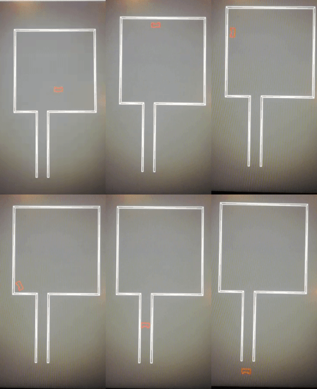
Before going for the final challenge, the wall-follow algorithm has been tested using a trial map with corridor width set to the lower limit of 0.5m. As can be seen from the video below, the PICO has successfully made it through the narrowest corridor in the trial with this strategy.
Challenge results
With the wall-following algorithm, the PICO achieved second place in the escape room challenge. The exit was reached within 27 seconds. The result of the challenge can be seen in the video below. With the created algorithm, it can be seen that PICO firstly moves to the wall in front of him and stops when he is within the threshold range. After this, PICO perfectly aligns himself perpendicular to the wall, ready to move to the left. When moving to the left, first it encounters a convex wall, which means he rotates and aligns to the wall left of him. After the PICO is aligned to the new wall, it moves to the left until it encounters the corridor. Here, the PICO positions himself in front of the corridor. Once the PICO is positioned and feels it is safe enough to move, it drives through the corridor to the exit.
Evaluation
Initially, the plan was to use fastSLAM to detect the corridor and let PICO drive to the corridor from its initial position. However, this did not work out as intended because there was not enough time to finish the fastSLAM code before the escape room challenge. For this reason, a wall following algorithm was created as a second-best option to let PICO escape safely and quickly. Some features were added to the wall following algorithm that makes it an upgraded wall follow algorithm suited for the escape room environment. Features such as concave and convex corner detection and exiting through the corridor without collision made it challenging, but as can be seen in the escape room challenge result section, the created wall follow algorithm worked as intended and let the PICO escape the room within 27 seconds having the second-fastest time of the challenge.
Hospital Challenge
The software architecture for the Hospital competition is explained first. A detailed description of the class diagram is given together with a list of the implemented algorithms. An explanation of the different implemented algorithms is given in the next section. After this, the difficulties are listed. The results of the hospital competition and own trials are discussed in the next section. Lastly, an evaluation is given on the coding process.
Software Architecture
The software design is explained in this section. An overview of the structure of the software is given and the different functionalities are listed. Such that the overall structure and connections in the software are clear. A detailed explanation and reasoning of the individual algorithms are given in the next section.
The software design is based on the different challenges that occur in the Hospital competition. This means that all the challenges, that at first sight can be deducted, are listed before a design is made. [I dont understand this sentence, why not just completely remove it -Max]
To complete the hospital run the PICO should be able to plan a path between two given points. The path should be based on a map. The two given points, start and goal, are defined as a coordinate in this map. For this functionality, pathfinding, a costmap-based algorithm called A* is used.
The translation between the coordinates in the map and the real coordinates in the hospital should be constantly monitored. The relationship is not direct, because the odometry data has noise. This implies that this translation can not purely be based on odometry. On top of the odometry data, the LRF data can also be used to deduce the position of the robot. However, there is also noise present in the LRF data, so a combination of the odometry- and laser data should be used to deduce the position of the robot. A FastSLAM algorithm is used. This algorithm makes use of different landmarks in its surroundings. An algorithm to spot and link the local landmarks to the global landmarks is needed. A feature-detection algorithm is needed to accomplish this.
Based on the localization and the calculated path, the PICO should be able to move from its current position to a defined next position. During the movement, static and dynamic objects should be avoided at all times. A velocity-vector based algorithm can take this active avoidance into account via a so-called potential field.
The main algorithms of the software are A* algorithm for Pathfinding, FastSLAM for localization and orientation, velocity vector for path movement, a local potential field for obstacle avoidance, a feature detection, and a mapping procedure. These algorithms are the foundation of the whole software and the designs are based on these algorithms.
A class diagram is made to give an overview of the general structure of the software. The different above mentioned algorithms are grouped to form a class, with the intention to create a hierarchy. The supervisor class is created as the top class in the hierarchy structure. In this class, every other sub-classes are called. The supervisor class is divided into 5 modes, namely initialization, scout, move, wait, and act. Switching between these modes is done on the basis of the outcome of the function in the sub-classes.
The sub-classes that are directly underneath Superivsory are Navigation, FastSLAM, and Visualization. The abovementioned algorithms are divided into these sub-classes. The Navigation contains the A* global path planning, velocity vector based movement, a local potential field, and feature detection. The Navigation class has a sub-class named Interaction, which is the only connection point to the PICO robot. The reading of the sensors and the control of the movement takes place in this class. However, since these readings are needed in other classes a struct is made, which contains all the useful information based on the current readings. This struct is made in the supervisor class and is linked to the address of a similar struct in the Interaction class. The current readings and detected features are now available in the supervisor class and can be from there. The FastSLAM class is a class fully based on the FastSLAM algorithm with a sub-class Particle which plays an important part in the algorithm. The Visualization class is based on the visualization and maintaining the map of the environment.
Due to the iterative process nature of a robot, the software is also designed on this bases. Every iteration starts with sensor reading and pre-processing of this data. The sensor data consists of laser and odometry data. The pre-processings part, processes the raw sensor data in such a way that it is usable for the next processing part. The data is now usable for the main step in the iterative process, the so-called processing step. The pre-processed data is the basis for the different algorithms, that are run in this part of the process. The outcome of the different algorithms are stored and are available in the next iteration.
Course Paradigms
In the tutorials page on the CST Wiki, an example of a software architecture that can perform some robot functions is given. This consists of Worldmodel, Detection, Drive Control, Configuration, and Main files. They are just meant as an example of an architecture that has different classes interacting. They could have been used as a basis for our architecture. However, it was decided to organize our system along with the main tasks that needed to be performed. This did not coincide with the example.
Algorithms
For the Hospital Challenge, the design of the algorithm is divided into four parts: interaction, supervisory, mapping and navigation. Each part has its own functionality and needs to work with the other parts. This functionality is explained below:
Feature Recognition
The goal of the feature recognition part of the software is to read PICO’s laser rangefinder data and interpret it in a way that is useful for the localization algorithm.
The first main function is to detect corners. The hospital consists of perpendicular straight walls. The localization algorithm uses the corners of these walls as landmarks. The rangefinder data is divided up in a number of straight-line segments for the walls. The ends of these segments are, after a filtering step, seen as corner landmarks and saved.
The second main function is identifying the corners. The localization not only needs to know what corners PICO sees but also which corners those are. The supplied hospital map has a numbered list of the position of all corners. Using the PICO’s position the detected landmarks can be matched to the map landmarks and obtain their ID.
The feature recognition consists of the following algorithms:
- Dividing the data points into segments
- Designating the ends of segments as detected landmarks
- Filtering the detected landmarks to reduce the matching workload
- Matching the detected landmarks to the map's landmarks
Segmentation
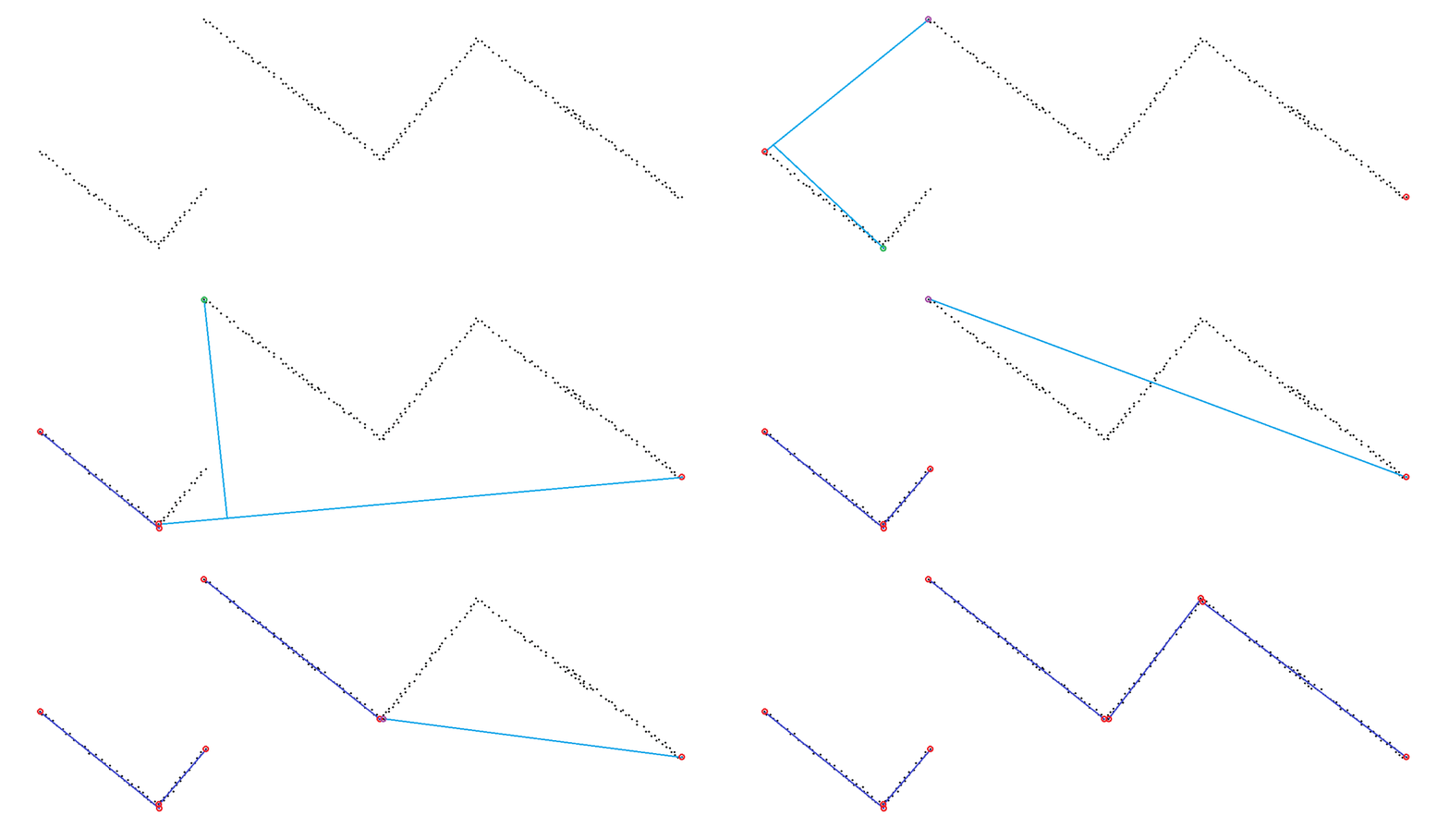
The detected laser rangefinder data consist of an array containing 1000 radii, the corresponding angles of these points as seen from PICO are fixed quantities. Together they make up a local polar coordinate system. The segmentation algorithm uses these points in cartesian coordinates so a conversion step is used.
The algorithm starts by considering all 1000 points as a prospective line segment with the first and last points as the start and end. Then for every point in between, it determines the orthogonal distance to a line spanned between the endpoints. While iterating the point with the largest distance is remembered. If the farthest point is closer to the line than a certain threshold a definitive segment is found and added to the list of segments. If the point is farther away than the threshold it is used to split the prospective segment.
The new prospective segment has the same first point, the last point has been changed to the farthest point found before. The algorithm iteratively splits the prospective segments this way until a valid one is found. Then a new prospective segment is considered. The first point of this is the one at the end of the previous segment, plus one. Segments do not share points, this is done to account for gaps in the walls. The last point of this segment is again the 1000th point.
The segmentation algorithm is demonstrated in Figure [segmentation_figure].
The algorithm continues splitting segments and adding them to the list until the endpoint of a definitive segment is the 1000th point. Then the end is reached.
The code implementation uses two methods: individualLineSegmentation() receives the start and endpoints of a prospective segment and determines if it is a valid one, and if it isn’t it returns the point that is farthest from the line. LineSegmentation() receives the output from individualLineSegmentation() saves valid line segments and determines the next prospective line segment.
 Segment FeatureExtraction::individualLineSegmentation(int range_start,int range_end)
 {
   float d =0, x_diff, y_diff, x2y1, y2x1, d_max =0, i_max=0;
   int max_features = 50;
   int line_end;
   x_diff = curCarEnvelop[range_end].x-curCarEnvelop[range_start].x;
   y_diff = curCarEnvelop[range_end].y-curCarEnvelop[range_start].y;
   x2y1   = curCarEnvelop[range_end].x*curCarEnvelop[range_start].y;
   y2x1   = curCarEnvelop[range_end].y*curCarEnvelop[range_start].x;
   for(int i = range_start; i<range_end; i++)
   {
     d = fabs(y_diff*curCarEnvelop[i].x-x_diff*curCarEnvelop[i].y+x2y1-y2x1)/ sqrt(y_diff*y_diff+x_diff*x_diff);
     if (d> d_max)
     {
       d_max=d;
       i_max=i;
     }
   }
   if (d_max<threshold_linefit)
   {
     Segment x(range_start,range_end);
     return x;
   }
   else{
     Segment x(i_max,-1);
     return x;
   }
 }

 void FeatureExtraction::LineSegmentation()
 {
   conversionCartesian();
   segmentRanges.clear();
   float startR=0 , endR=999;
   int index = 0;
   bool notDone=true;
   while(notDone)
   {
     Segment segment(individualLineSegmentation(startR,endR));
     if (segment.endR == 999)
     {
         notDone=false;
     }
     if (segment.endR == -1)
     {
         endR = segment.beginR;
     }
     else
     {
         segmentRanges.push_back(segment);
         startR=segment.endR+1;
         endR=999;
         index++;
     }
   }
 }
Line Fitting
The segmentation algorithm only finds the first and last point making up a wall, the measurements for these contain noise. To mitigate that noise a line is fitted through all the points making up the wall segment. This is done using a Total Least Squares regression. This looks at deviations in two directions and fits a line that minimizes the orthogonal distance between the points and the line. Later when filtering the features, the intersection between two lines can be used as a better estimate of the corner position.
During debugging it turned out that an increase in accuracy was not needed and this method was skipped in the end.
Landmark Creation
A struct of landmarks is created that consists of all the points at the ends of the segments.
Corner Detection
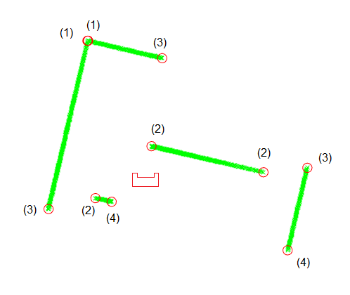
The landmark matching algorithm used later computes the distance between all detected landmarks and all the landmarks in the hospital map. However, only about half the detected landmarks denote actual corners. In general, PICO sees between two and around 15 segments, 30 landmarks. Excluding moving objects, the hospital has 115 landmark corners. With n detected landmarks and m map landmarks, matching is an O(n*m) operation. This corner detection is an O(n) operation that halves the number of landmarks passed on.
There are four types of landmarks that PICO can see:
- A corner that is seen in its entirety.
Here two segments meet and two landmarks are close together. Only one landmark is needed and the midpoint between the landmarks is saved.
- A corner that is seen from one side and inferred.
- The end of a wall’s observation caused by occlusion.
These two exist when one wall is in front of another. As seen from PICO there are two landmarks close to each other in angle but far apart in range. The landmark farthest from PICO is not a corner, PICO just doesn’t see the end of the wall. The closest landmark is an actual corner and is saved.
- The end of a wall’s observation caused by PICO’s blind spot.
The first and last landmarks are not corners but again the end of PICO’s observation of a wall.
These different detected landmarks are illustrated in Figure [detected_corners].
The method used, computeVisibleLandmarks(), iterates with a step size of two over the landmarks and compares them to the next in the list. This way only sequential landmarks belonging to different segments are compared. The comparison checks if the pair of landmarks are close together, if so it indicates they are type (1) and adds the midpoint between the two to a new list of landmarks. If not it checks if the pair makes a set type (2) and type (3), if so it adds the closest one to the list. The first and last landmarks are always skipped.
This method is not essential for functioning, it makes another computation faster. Due to some debugging problems this method was skipped over in the end.
Corner Identification
All the landmarks in the hospital map have a numbered ID. The goal of the method labelLandmarkIDMatched() is for every detected landmark to find the map landmark that corresponds to it and copy its ID. The method iterates over the detected landmarks. For each detected landmark it then iterates over all map landmarks and computes the distance between the two. If that distance is smaller than a certain threshold a match is made
The coordinates of the detected landmarks are all from the point of view of PICO. With the method transformationLoToGo() they are transformed into the coordinate system of the map using the latest estimate of PICO’s position and rotation.
Closed door detection
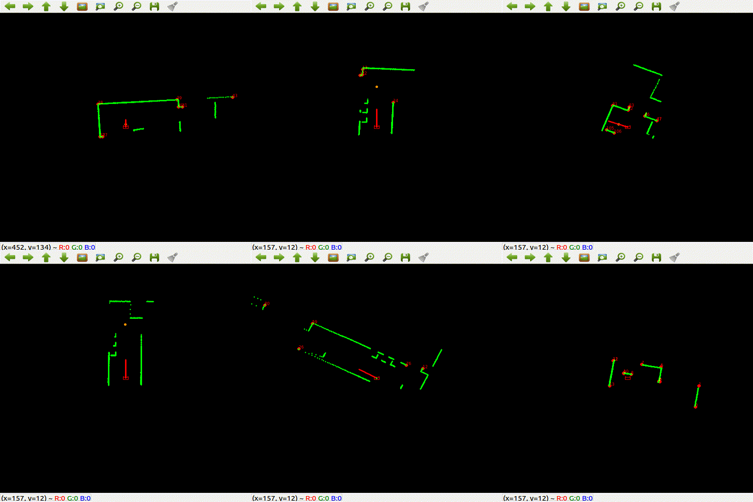
The dynamic and static changes that occur in the hospital environment needs to be captured on the global map. A closed-door is one of those changes. Detecting this change is needed since driving through a door is not desirable. Therefore an algorithm to detect a closed-door is implemented.
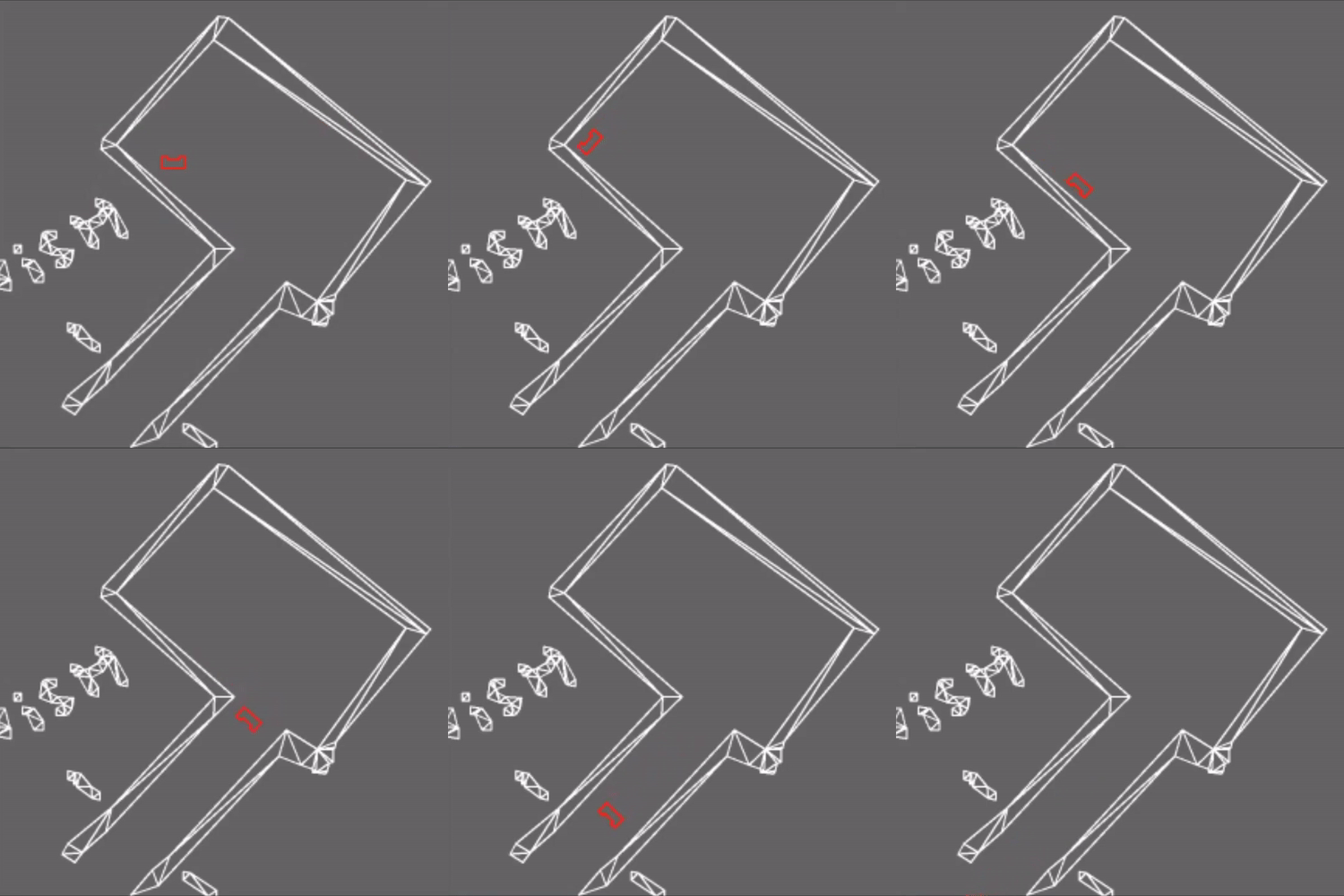
The algorithm is called when the desired velocity vector and the contrary vector, based on the local potential field, results in vector with a near-zero amplitude. This implies that the PICO is positioned in front of a door, which will trigger the door detection. At the start of the program, a map is made on the basis of a JSON file. On top of the labeling of the different landmarks and grouping some of them to form a cabinet, some of them are grouped to form a doorway. Since the position of the robot is known when the door detection algorithm is triggered, the vector of the current position to each of the doorways is calculated. The smallest vector is the doorway that is in front of the PICO. Adding this so-called wall to the vector<Wall> variable will result in adding this wall to the global map. Due to this change, the cost map is updated, which will result in a different A* path. In this way, the closed-door is mapped on the global map. The following figure shows the visualization of the current envelope when a closed-door is detected.
Visualization
The visualization of the different algorithms is used as a way to check the correctness of the outcome. In total there are three different visualizations, the global map, a costmap of the global map, and the current envelope. The global map is used to check if the robot is correctly orientated. This is done by plotting the seen landmarks in the current envelope on top of the global map. If the local landmarks overlap with the global landmarks, it implies that the robot is correctly orientated.
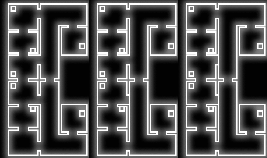
The costmap functions as a basis for the A* algorithm. If the costmap is not correctly defined the A* algorithm will not function as desired or not at all. The costmap is a blurred and tiled version of the global map. Convolution with a gaussian kernel is used to blur the global map, which leads to a valley like distribution in a room. This distribution is desired since this will lead with the A* to a path that goes straight through the middle of a room or hallway. The white color represents a wall where the PICO cannot go through, and black is the space the PICO can move freely. The blurriness of the white represents the cost of the map. The sharper the white color, the higher the cost. The envelope shows the current laser data with the labeled landmarks from the feature detection. The labeling of the landmarks is checked via this visualization and is shown in the following video.
FastSLAM2
In order to describe FastSLAM2, as well as the choice to use it, we will use deepening steps from the overall problem of SLAM, through the generic strategies to solve it, down into the algorithm itself.
The SLAM Problem
To solve the SLAM problem is to answer the age-old questionWhat came first, the chicken or the egg?
In less symbolic language, let's put it this way: during operation of the robot, in almost every timestep k ∈ ℕ, we attempt to answer the question 'Where are we?`, which implicitly contains two much more concrete questions;
What is my position, relative to my surroundings?
What are my surroundings and their meaning or position relative to me?
Without any mathematics involved, one can already start to see an emerging intrinsic relationship between the localization problem and the mapping problem.
Certainty cannot be achieved during timestep k, and as such, the art is to get as much certainty as is possible without exceeding a bearable workload, so we don't find ourselves too computationally burdened to be ready for the next timestep. There are many ways to cope with this problem, from the simplistic `not dealing with it at all`, using a Zero-Order Hold (ZOH), or a ZOH with the inclusion of the proposed movement and positions from the current timestep, all the way to the rather absolute, offline `GraphSLAM` method, which saves countless measurement points, and tries to optimize the sense these points make relative to each other (or: attempts to minimize the magnitude of discrepancy between measure points).
Our problem is marked by being online (PICO needs to know what's going on while it's happening) in a rigid environment, under uncertain starting conditions, with noisy motion and noisy measurements. PICO additionally has to deal with random, dynamic elements, which one could attempt to deal with in the SLAM module of a program, but we won't, simply so we can keep using a rigid world assumption. Instead, the workload for coping with dynamic elements will be on feature recognition, which will have to make the judgment call to name a random element static (and add it to the map of rigid elements) or dynamic.
In the world of online SLAM methods, we will very quickly find ourself submerged in the world of world features considered through Extended Kalman filters (EKFs), and since we have noise (or: a constant threat to localization certainty), as well as an uncertain starting position, we will also find ourselves looking to use a particle filter as to not find ourselves locked into a single wrong hypothesis.
This brings us to the next section, where we will explain what the inner workings of an EKF particle filter are.
Simultaneous Localization and Mapping using Particle Filters
In this section, we will expand on the basis given by the course lectures. Most additional knowledge here is derived from the (freely available) lectures on SLAM by Cyrill Stachniss, a full-time professor at the University of Bonn.
The Particle Filter Side
Let us consider first the particle filter side of our fledgling concept of SLAM. Each particle within the cloud of n particles represents a hypothesis, containing within itself a presumed location (x,y) of the platform - PICO - and its assumptions about the surroundings - the EKF part of the problem. With each update, these hypotheses are somehow updated under assumptions about the predicted motion since the last timestep and under the interpretation of the measurements received in the current timestep. The idea is that if the problem is observable and noise is adequately respected, the cloud of hypotheses will continuously converge on a correct solution, giving a supposedly ever-sharpening fuzzy localization that can be adequately used as a substitute for a true notion of the platform's pose (location and rotation) in the world.
The crux of a particle filter solution is to somehow weight assumptions with measurements. To keep things formal, let us steal a little part of the EKF side of the problem, and already introduce the concepts of a prior (the assumed position) and posterior evaluation (the expected position based on measurements). This, formally, gives us the following primary mechanic to work our particle filter with:

Armed with a definition for the weight (or 'belief') we give a certain hypothesis, we can talk about the workings of our particle filter. After every timestep, every particle - and thus every hypothesis - has been given a weight; these weights have meaning relative to one another, and for the sake of keeping the risk of binary overflow errors to a minimum, these are linearly normalized somehow relative to some measure - e.g. the sum weight or the maximum weight.
We now steal a page from the concepts constituting machine learning; we cull hypotheses that are too weak and let the likely hypotheses dominate the cloud. That is: some particle's respective weights, after normalization, are weaker than some minimum parameter, and so these hypotheses are destroyed. After this, we somehow decide whether our hypothesis population is underpopulated, and repopulate it with n_new new particles based on the pool of hypotheses we currently have during a resampling process. This resampling process is best described as spinning a wheel, where the portions allocated for particular particles on this wheel are scaled depending on their weights.
Literature suggests that low-variance resampling is the way to go here, which is an algorithm that is often instead called 'roulette wheel resampling'. The idea is that normal spin-the-wheel-with-every-pick resampling has a (completely unnecessary) chance to arbitrarily favor a particular group of hypotheses by repeatedly picking their members as resampling candidates. Roulette wheel resampling instead spins the wheel once, and then jumps around the wheel n_new times, with jumps scaled by the total weight of all particles, divided by n_new.
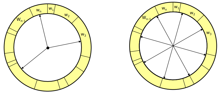
The above picture, from Stachniss's slides on probabilistic robotics, is a clear illustration of the normal pick-every-sample algorithm (left) and the roulette wheel approach (right). Note that, additionally, the simple approach has algorithmic time complexity O(n log(n)), as every sampling also needs to be looked up by index in the particle list, whereas the roulette wheel approach does lookup intrinsically as part of generating the 'spokes' of the wheel, and hence has algorithmic complexity O(n).
This concludes the particle filter side of our understanding of SLAM. In one pseudocode block, let us summarize the core concepts before we dive into the ugly side that is Gaussian predicates:
Cloud particleFilter(Cloud particles, PredictedMotion u, Observation z) {
   for each particle in particles :
      particle = updateParticle(particle, u, z);
      // To be defined in the EKF side of things.
      // This step already updates the weights, but let's make it explicit.

      particle.w = updateWeight(particle, z);
      // Evaluate assumptions based on observations.

   particles = normalizeWeights(particles);
   particles = cullWeakHypotheses(particles);
   particles = lowVarianceResample(particles);

return particles;
}
Given that we have some functional way to predict our behavior and rate a hypothesis, and have made adequate decisions in defining our prior and posterior weight factors, we now have a particle filter that will continuously converge to an optimal hypothesis, without locking itself into a particular belief. In other words, we have described a learning algorithm that looks to minimize the localization error but won't decide on a certain group of hypotheses until it gets evidence that sways it one way or another.
But we do not have the necessary mathematics in place yet, so... let's get that over with!
The EKF Side
This part leans heavily on the aforementioned lectures, and the research papers 'FastSLAM' and 'FastSLAM2.0' by Montemerlo, Thrun, Koller, and Wegbreit.
For the mathematically intensive part of this problem, we will be dealing with probabilistic distributions and laws, such as p(s(k+1) | u(k+1), s(k)). This reads as 'the probability that we will see a certain pose s(k+1) at time k+1, given that we saw s(k) at time k while we've been told we moved with a vector u(k+1) this timestep.' To be precise, this particular distribution is already important enough to be denoted as an equation!

What we have just described is known as the probabilistic law that describes a motion model. To be more precise, assuming that u represents a shift in pose (rather than a vector of velocities), and both state vectors s represent robot poses (x, y, θ), and no outside influence, the average position of the robot will be s(k+1) = s(k) + Au(k+1).
As we have already discussed the particle filter side of things, this is also where we need to introduce the concept that our position shifts u(k) are noisy. In order to make our probability distribution truly a distribution, the idea is to have each particle updated both strictly with u(k), and with a random amount of process noise Q.

Where random generates a vector of 3 elements given random values according to the normal (float) distribution with mean 0 and st.deviation 1. Note that Qprocess is a representation of the noise in PICO's odometry, and hence a correct value will have to be measured, obtained from simulation settings (as a substitute to experimentation), or approached through tuning. As it is a compounding problem to try and dynamically calibrate noise covariance, this is out of consideration due to complexity alone - it would be like bringing another two smaller SLAM problems into the original SLAM problem.
The result of implementing (3) is that our particle filter - without any further logic - is an n-sampled representation of the motion law (1). Each timestep has the particles of our cloud spread out further while adhering to the dynamics of u with each timestep. In other words, (3) implemented into a particle filter is an answer - but not a good answer - to the question `Where is my position, relative to my surroundings`.
Now we consider the other probabilistic law in SLAM, which just so happens to answer the other question posed at the start of this section;
Where we need to quickly introduce the concept of a landmark or feature. Within the confines of this project, it suffices to say 'corners', but in a more general sense: a landmark or a feature is something that the robot's sensors and feature recognition software can spot. Ideally, this is something that a robot can reliably and somewhat precisely pick out from its surroundings, but that is not formally part of the definition.
The law in (4) is known as the measurement model in literature. It talks about the probability that we make an observation z at time t, given that the robot has pose s(t), lives in the world w (which is a list of landmarks/features the robot can see), and that it has had some correspondence h(t) (which is an identifier for a certain landmark that is suggested to have been seen by the observation z). In other words, it is an answer to the question `I think I saw this. Should I see this?`, which is directly related to `what are my surroundings, and what are they relative to me?` when we apply it to more than a single observation. We're almost there!
Note that we have not introduced any notion of persistent landmarks; the set w can theoretically expand infinitely. The reason that this matters will become apparent shortly when we combine the two probabilistic laws (2), (4) into a probabilistic definition of our SLAM problem:
Note that we now have superscripts t; this notation means 'from time t0 up to time t'. In normal English, (5) poses the question `How likely is it that I am here, and the world is what I think it is, given my prior observations, given the motion I've undertaken, and given the landmarks I've spotted?`. In even more normal English, this reduces to `Given that I've seen these things, am I right to think I am here?`.
If you'll remember the concept of weight from the particle filter side of things, this is the notion used to weight a certain observation. This probabilistic law is sufficient to set up an algorithm to localize a robot in a world with a limited amount of potential features, but as the process involves at least one inverse, and this inverse is currently tied to the size of the set w, this is very easily going to become computationally infeasible. This is where we move on to the fastSLAM part, where we will finally fill in the actual methods to turn probabilistic law into quantifiable outcomes.
FastSLAM and FastSLAM2
As a small recap, we have introduced the concept of a particle filter serving as a cloud of hypotheses, or guesses, to the robot's position, and the idea of probabilistic distributions that we can use to evaluate the feasibility of a certain measurement given a certain hypothesis and history.
The core idea that makes FastSLAM so powerful is its exploitation of the given fact that landmarks are static. This is best put in the following observation:
If we know the path of the robot, landmark positions can be estimated with respect to the robot, independently from one another.
This takes the form of another probabilistic law:

Where lm represents a particular landmark in the world set w, and mᵗ is the weight factor history of a certain landmark. In other words, we've here refactored the problem (5) into two much (computationally) lighter subproblems; that of the likelihood that the robot has a certain pose, and that of the compounded set of likelihoods that a certain landmark is seen the way it has been seen, if it has been seen, at a given time.
The reason that this matter is that the processes of updating and evaluating the measurement model involve inversions of covariance matrices with a size equivalent to the world set, plus the 'moving landmark' that is the robot itself. Inversions are an O(n³) operation.
In (5), the world set is the combined set of all landmarks, which in the hospital challenge by default were already in the order of 100 points; 100³ operations, every single iteration, for every particle and every correspondence, is a gigantic workload. In (6), however, the world set(s) is (are) much smaller; it is the local world of the considered landmark, which can be described through a mean position and, with PICO included in the equation, a 2x2 covariance matrix. 100 times 2³ is much, much smaller than 100³.
This allows us to formulate our particle filter as a system of n particles with m small internal models, one for each landmark in the global map. Each internal landmark model lm is stored with global coordinates, but a local origin; it describes a mean distance in (x, y) to the particle in question, with a covariance H describing how certain that mean is. This is compounded with a measurement covariance R that is used to account for measurement uncertainty.
This brings us to the basic operation of the FastSLAM algorithm, in pseudocode:
void FastSLAM(Cloud cloud, PredictedMotion u, ObservationSet zt){
   for each particle in cloud {
      // Predict
      particle.updatePose(u); // as per (3)

      // Observe
      for each z in zt {
         if(particle.lm[z.id].known)
            particle.updateLandmark(z);
            particle.w *= getWeight(z);
         } else {
            particle.lm[z.id] = particle.newLandmark(z);
         }
      }
   }

   // Adapt
   cloud = cullHypotheses(cloud);
   cloud = resample(cloud);
}
Where we implicitly also added an intuitive boolean evaluation of whether the robot has yet encountered a certain landmark. We have, however, yet to define the behavior of making, updating, and evaluating landmarks. Given that an observation z is an LRF-measured landmark, represented as the tuple LRFLandmark(int id, float r, double th), we will first tackle the easiest of those to-be-uncovered elements in makeLandmark. Note that a particle contains its pose as a vector p = (x, y, θ), and that a landmark is represented as the tuple Landmark(int id, bool known, float x, float y, Matrix2f H, where known is set to false at initialization, and true forever after makeLandmark(), and a Matrix2f is a 2x2 matrix of floats (from the Eigen3 library).
Landmark Particle::makeLandmark(LRFLandmark z) {
   Vector2f pol2car_g = [cos(z.th + p[2]); sin(z.th + p[2])] // p[2] = robot angle
   Vector2f d         = z.r * pol2car_g;

   Matrix2f jacobian  = [
      d[0]/z.r,       d[1]/z.r;
      -d[1]/(z.r^2),  d[0]/(z.r^2)];
   Matrix2f invJ      = jacobian.inverse();

   Landmark lhs;
   lhs.id    = z.id;
   lhs.mean  = p[0:1] + d;
   lhs.H     = invJ * R * invJ^T;
   lhs.known = true;

   return lhs;
}
Note that this pseudocode used a more matlab-esque notation for matrix and vector formatting than C++ uses. For further uses of the jacobian of a vector d and a range r, we will instead make use of Matrix2f getJacobian(Vector2f d, float r).
Path Finding
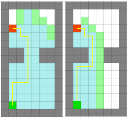
For pathfinding, A* is chosen. A* is a pathfinding algorithm-based and built on Dijkstra's Algorithm. Dijkstra's Algorithm looks at every available cell all around the start point, until it reaches the goal. This algorithm uses a costmap to find a proper and efficient path. A* has the same function as Dijsktra, but is smarter, and attaches more value to the cells towards the goal. Because of this, A* needs fewer iterations and is faster. This difference can be seen in the images below, where Dijkstra's algorithm is in the left figure and A* in the right figure. The difference is even more noticeable as the map gets bigger.
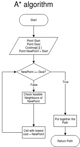
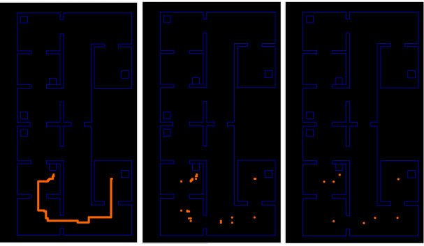
And thus an A* algorithm is made, where the working of the algorithm can be seen in A* code snippet and is explained in the flowchart on the right. The A* function needs a costmap, a start point, and a goal point, and based on this it makes a path. Every time the PICO reaches a new cabinet, a path is generated to the next cabinet. A reduction path function is added, which takes the output path of the A* pathfinding function, and removes all of the points which are in the same direction. This ensures that only the important points which need to be reached are left. Also, there is an option in the reduction path function to cluster points that are closer together. With the local potential field (which is further explained in Path Movement) the PICO can move safely even if some points are clustered together. These clustering of points are displayed in the image below, where the first picture displays all of the point returned by the A* algorithm, and thus it got a huge amount of point close to each other. The second image only displays the last point of the same direction of a path. The third image reduces the path even more by clustering points in a specific range.
Path Movement
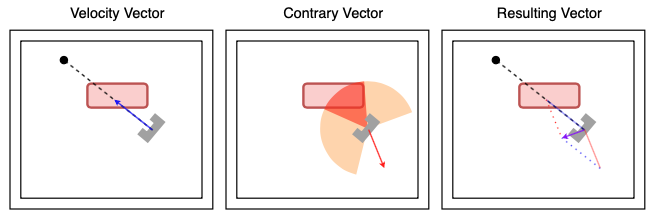
Path movement translates the points of the trajectory of the A* algorithm to a vector of necessary x and y speed values for the PICO robot to follow the trajectory. To make the path movement smoother, and as security for the PICO, a local potential field is used. Based on the objects or walls in a defined range, the PICO generates a contrary vector. The velocity vector and contrary vector together creates a resulting vector, which determines the actual movement direction of the PICO. When the PICO is in a given range of the point it needs to reach, the pico goes to the next point in the path vector, which is put together by the A* pathfinding function.
Course Paradigms
Lecture 3.3 on Motion Planning makes a division between global and local planning. In our implementation, this is also used. The A* algorithm decides a path through the entire hospital. The potential field algorithm improves the local smoothness of the path and improves the obstacle avoidance. A number of map decompositions of the map are shown, a visibility graph, a Voronoi diagram, and a cell decomposition. The hospital consists of rectangular static walls (with some moving objects) which suits the easier implementation of a cell decomposition. The considerations of how to handle a cell being seen as not completely occupied or free are taken into account. Another example is the global potential field, this has an attractive source at the destination and repulsive sources from obstacles. This can run into problems with local minima. Only a local potential field implementation was deemed necessary.
Results
The result of the hospital challenge can be seen in the video below. Unfortunately, the fastSLAM did not work as intended which led to the PICO robot not having an accurate idea of its current position and the environment. This made it impossible for PICO to move along the created trajectory and thus failed to complete the hospital room challenge.
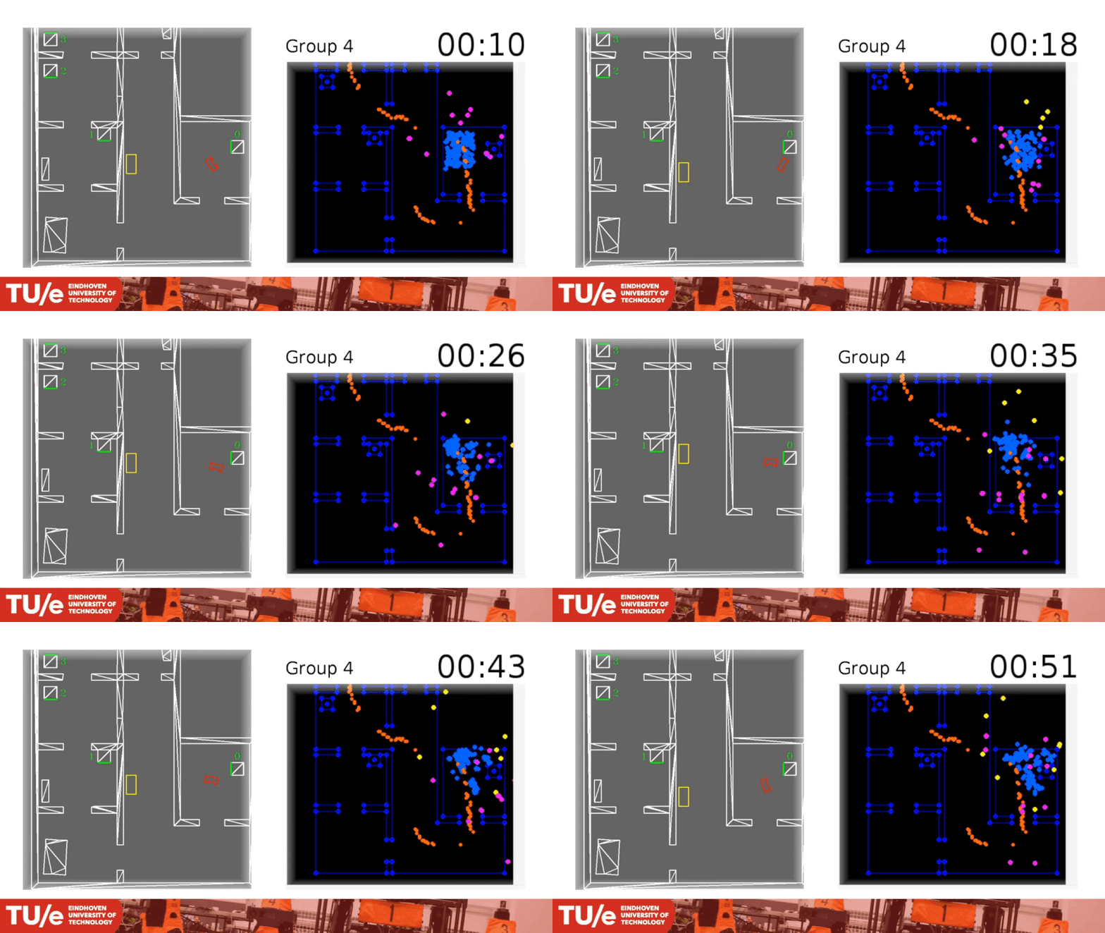
After a lot of time and effort, we were unfortunately not able to implement the fastSLAM algorithm as intended, resulting in a PICO that moves purely based on no-noise odometry. Since most of the other functionality does work, the hospital challenge is done with no-noise odometry. In this way, it is possible to show a working robot.
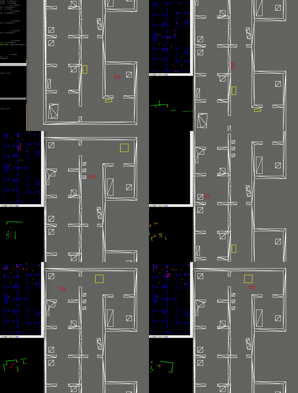
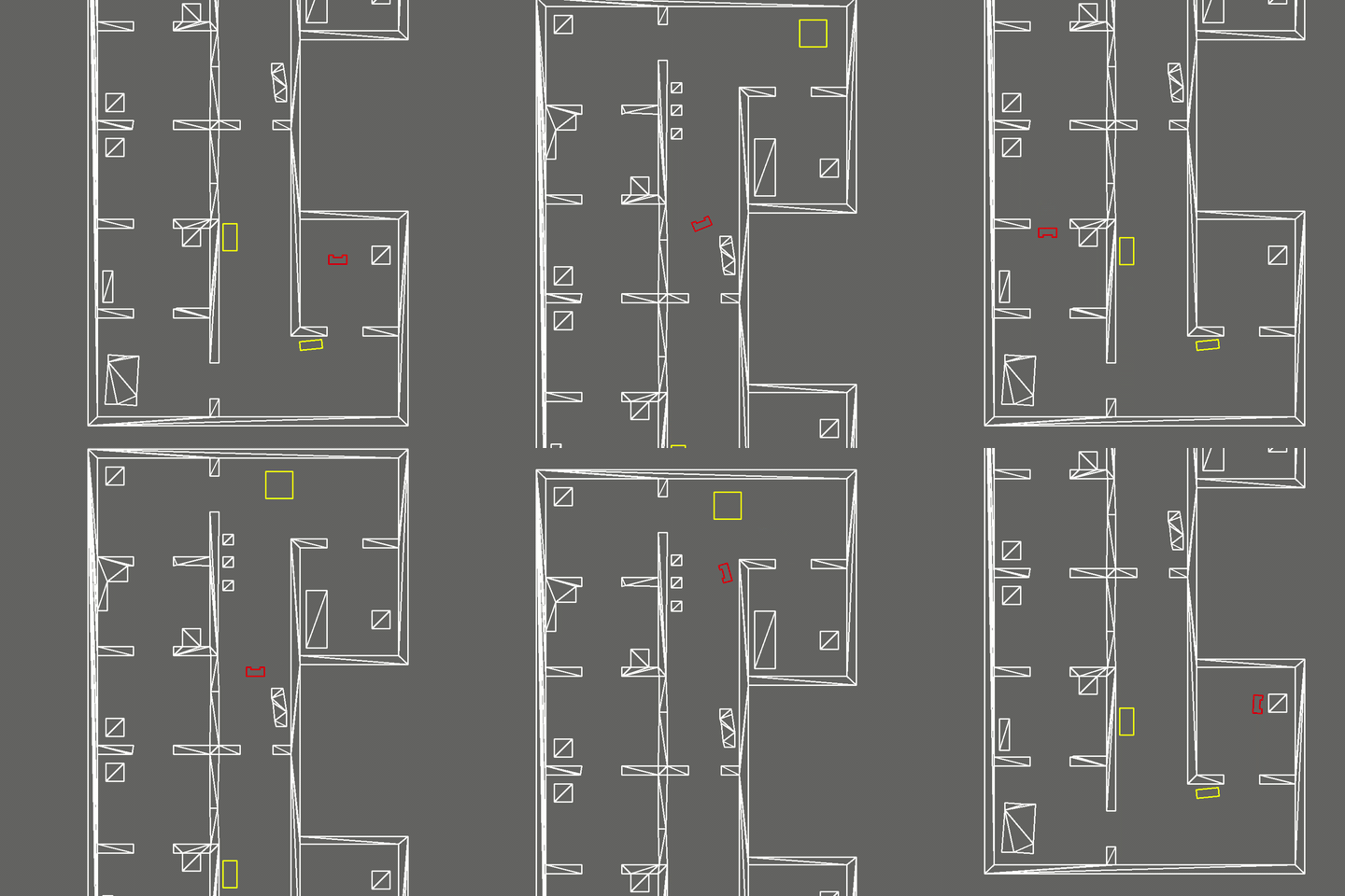
The code doesn't take into account the static and dynamic objects in its path planning. This is unfortunately visible in our own hospital trial. Since we want to show every functionality of the PICO, the path of the different cabinets is changed to (3,1,6,0).
Difficulties
FastSLAM2
The foundation of SLAM, considering its usage of probabilistic laws and, as one paper put it, rich pre-existing literature, was difficult to grasp. As such, error catching was a difficult process, caught between the usual attempts to trace missing minus signs and the like, grasping at variables that, through the network of equations between one state and the next, could potentially be the cause for some sort of error, while also always being at risk that the implementation itself was simply incorrect.
Costmap
Another difficulty is that the cost map is created based on the initial map given and is only updated when a door is found to be closed. However, in the demonstration, random objects are placed or can even move around. The costmap does not get updated based on these objects. The A* pathfinding algorithm will therefore not adjust its path and wants to move through obstacles. This problem is partly fixed by using a potential field next to the path movement, but still has a problem with unfeasible waypoints, which is discussed in de evaluation section.
Coordinate transformation
Due to the three different coordinate systems, local-, global-, and pixel coordinate system, multiple transformations are needed to transform a point between the three coordinate systems. These transformations were initially done at the end of an iteration, just before when the transformation was needed. This resulted in a hectic mess. Since it wasn't clear at what point which coordinate system was used. Therefore a different approach is implemented. At the beginning of each iteration, the points were transformed into the different coordinate systems. These are then stored in the curINPUT variable in the Supervisory class. This variable is a struct that contains three different vectors for the different coordinate systems. In this way, a function that needs a point in a particular coordinate system can directly access this without computing it first.
Evaluation Hospital Competition
This section does not read like a professional report. Look it over. -R
Im still busy with this section rn ..... ? -R
Path planning and potential field/movement
The path planning algorithm works when a complete initial map is given. Based on the costmap, the A* algorithm finds a path, and with a velocity vector, the PICO accurately moves to a given goal point. First, a problem occurred where the A* pathfinding function generated a lot of waypoints between the start and goal point. With a reduction function, those waypoints were reduced. In a later stage of the project, a contrary vector generated by the potential field was added, which ensured the PICO could move smoothly and safely. The only limitation was that the actual map could differ from the initially given map, which is explained in the evaluation of "Costmap in combination with dynamical objects", and that the algorithm lacked a way to catch unfeasible paths.
Structure of the code
What also went well, was structuring the code, which is explained fully detailed in the Software Architecture section of the Hospital Challenge. Although the code deviated from the initial design in the design document, the base structure is still the same. The code still consists of the 4 key sections which work together: Supervisory, Interaction, Mapping, and Navigation. Each section got its own functions, which belong to this section. This ensured that each class or function could be tested separately and problems could be quickly detected.
Costmap in combination with dynamical objects
Something which was not working properly in the code is the costmap. The costmap is generated at the start and only updated when a closed-door is found, and not based on dynamical objects which were added later in the map. As mentioned in the difficulties section, the PICO avoids obstacles by the potential field algorithm. This works properly, but there is an exception that has not been thought out well yet. The path of the A* pathfinding algorithm bases its path on the cost map (without the dynamical objects). So it can occur that one of the waypoints of the path is on top of one of the objects, which actually cannot be reached, and thus it will be in an endless loop where the PICO is pushed back by the contrary vector (potential field) and attracted by the velocity vector.
One way to fix this problem is to change the costmap dynamically based on what the PICO is seeing, and create a new path. Another way to fix the problem is to change the pathfinding algorithm so that it can sense an unfeasible waypoint, and change only the unfeasible waypoints while leaving the other points of the path unchanged.
FastSLAM2
Our first implementation, as it would have been used at the Hospital Challenge, was convergent, and clearly had some semblance of awareness with relation to its surroundings, but moved completely differently from PICO's actual motion. After attempts to 'fix' this disconnect went nowhere, a second implementation was made, which was somehow simply unstable instead, causing the robot to explode off of the screen to infinity within a handful of timesteps.
In short, the failure here was that the task was too difficult, and the workforce applied to it too small. As one of the other groups showed, a Zero Order Hold approach is functional, using a normal EKF particle filter and simply regularly updating and taking the full computational overhead of an inversion on the full world set covariance matrix. However, functional does not mean good, and while it would have been better in retrospect to build a simple filter first, and then develop a complicated filter later, the decision for FastSLAM over basic EKF is a well-considered one. Causing PICO to stand still regularly without any operational cause is simply inefficient.
Some things that could have improved the odds of success are as follows:
- The logic and mathematics for FastSLAM are more complicated to understand than they are to use. In retrospect, too much time was spent trying to comprehend, while all that was needed at the time was a prototype that could approach the desired behavior. Prototyping and simply pulling in other group members to discuss complications would have likely increased the odds of success more than the hours that were now spent puzzling out intricacies.
- The first implementation was obviously close to functional. In retrospect, regardless of the compounding frustration in debugging it, it was probably the wise choice to stick with it and see it through. That being said, there is probably some universe where this same discussion states 'we should have rebuilt it', so: this is speculation.
- Parts of the greater system were developed with a deeply rooted dependency on the OpenCV library. As installing OpenCV proved to consume a lot of time with no results for multiple members of the group, and this dependency prevented running simulations (and as such forced inefficient collaborative debugging sessions), this is a primary point of critique for a second try. A low-to-mid-level control system has no reason to be deeply dependent on a convoluted graphics library.
- The group had a small number of skilled programmers in the sense of coding in C++. It would have been useful if the course came with a drill course for this situation, as the result was such that the penultimate programming work could go nowhere else than be loaded onto the group members that had the experience or affinity for it.
List of Meetings
| Date/Time | Roles | |
|---|---|---|
| Meeting 1 | 01-05-2020
11:00 |
Chairman: Bas
|
| Meeting 2 | 04-05-2020
11:00 |
- |
| Meeting 3 | 08-05-2020
11:00 |
Chairman: Max
|
| Meeting 4 | 11-05-2020
10:00 |
- |
| Meeting 5 | 12-05-2020
10:00 |
- |
| Meeting 6 | 15-05-2020
11:00 |
Chairman: Dominic
|
| Meeting 7 | 18-05-2020
11:00 |
- |
| Meeting 8 | 22-05-2020
11:00 |
Chairman: Roel
|
| Meeting 9 | 27-05-2020
15:00 |
- |
| Meeting 10 | 29-05-2020
11:00 |
Chairman: Rob
|
| Meeting 11 | 02-06-2020
11:00 |
- |
| Meeting 12 | 04-06-2020
11:00 |
Chairman: Ananth
|
Links
These will probably be invite-based but a backup link could be useful.
Gitlab: https://gitlab.tue.nl/MRC2020/group4
Overleaf design document: https://www.overleaf.com/project/5eabeda72b3e4100010f8b40
