Mobile Robot Control 2020 Group 6

Group Members

Students (name, id nr):
Joep Selten, 0988169
Emre Deniz, 0967631
Aris van Ieperen, 0898423
Stan van Boheemen, 0958907
Bram Schroeders, 1389378
Pim Scheers, 0906764

Logs

This section will contain information regarding the group meetings

List of Meetings

	Date/Time	Roles	Summary	Downloads
Meeting 1	Wednesday 29 April, 13:30	Chairman: Aris Minute-taker: Emre	Introductionary meeting, where we properly introduced ourselves. Discussed in general what is expected in the Design Document. Brainstormed of solutions for the Escape Room challenge. Set up division of tasks (Software Exploration/Design Document).	Minutes
Meeting 2	Wednesday 6 May, 11:30	Chairman: Emre Minute-taker: Stan	Discussing our V1 of the Design Document with Wouter. Devised a plan of attack of the escape room competition and roughly divided the workload into two parts (Perception + world model and Strategy + Control).	Minutes
Meeting 3	Monday 11 May, 11:00	Chairman: Stan Minute-taker: Joep	Discussing what needs to be finished for the Escape Room challenge.	Minutes
Meeting 4	Friday 15 May, 9:00	Chairman: Joep Minute-taker: Bram	Evaluating the escaperoom challenge and the groupwork so far. Made agreements to improve the further workflow of the project.	Minutes
Meeting 5	Wednesday 20 May, 11:00	Chairman: Bram Minute-taker: Pim	Discussing towards an approach for the hospital challenge. First FSM is introduced and localization/visualization ideas are discussed.	Minutes
Meeting 6	Wednesday 27 May, 11:00	Chairman: Pim Minute-taker: Aris	Discussing the progress of the implementation for the hospital challenge. Discussed difficulties with localization and object avoidance.	Minutes
Meeting 7	Wednesday 2 June, 13:00	Chairman: Aris Minute-taker: Emre	Discussing the progress of the improved particle filter, suggestions on how to improve on the map knowledge. Discussed what is of importance for the presentation on June 3rd.	Minutes
Meeting 8	Wednesday 5 June, 12:00	Chairman: Emre Minute-taker: Stan	Evaluating the intermediate presentation and discussing the final steps for the hospital challenge.	Minutes
Meeting 9	Tuesday 9 June, 13:00	Chairman: Stan Minute-taker: Joep	Discussing the final things needed to be done for the hospital challenge.	Minutes
Meeting 10	Tuesday 16 June, 13:00	Chairman: Joep Minute-taker: Bram	Evaluating hospital challenge live-event and division of tasks regarding the wiki.	Minutes

Design Document

The design document, which describes the design requirements, specification, components, functions and interfaces can be seen here.

Escape Room Challenge

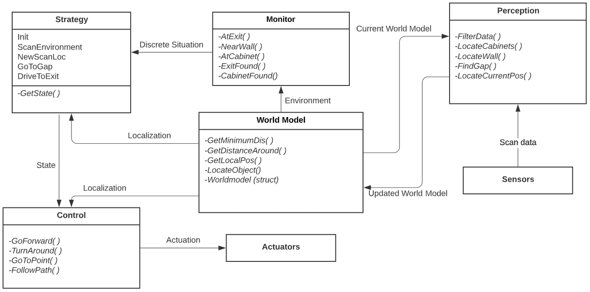
The escape room challenge required the PICO robot to escape a room with limited prior knowledge of the environment. The information architecture of the embedded software has been designed in the design document, the main components being: Perception, World Model, Monitor & Strategy and Control. The world model has been visualized using openCV which is available via ros.

Information architecture

Information architecture of the software during the escape room challenge

Perception

The objective of the escape room challenge is finding and driving out of the exit. To be able to achieve this, the robot should recognize the exit and find its location, which is the main objective concerning perception. For this challenge, the features of the room are only stored locally. The robot tries to recognize the exit, where after the location w.r.t. the robot is determined. First of all, unusable data points of the LRF sensor have been filtered out. A line detection and an edge detection functionality has been implemented in order detect the walls of the room in local coordinates. This way, at each time step, the begin point, the end point, and the nearest point of the walls can be observed by PICO. The functions work in the following manner:

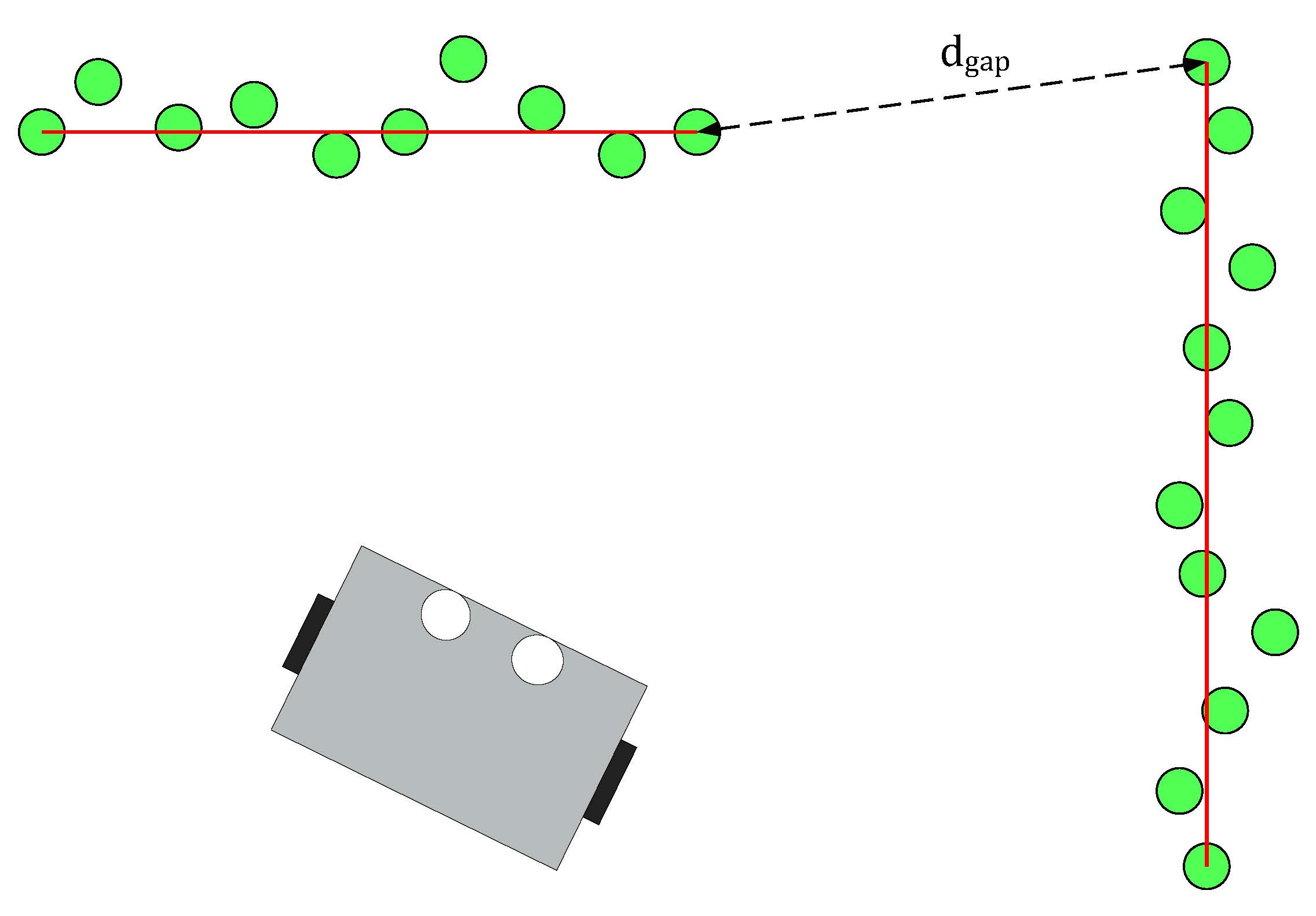
• Line detection: the LRF data consist of 1000 points with each a range value, which is the absolute distance to PICO. The line detection function loops over the data and calculates the absolute distance between two neighboring data points. When the distance exceeds the value d_gap, the line-segment can be separated.
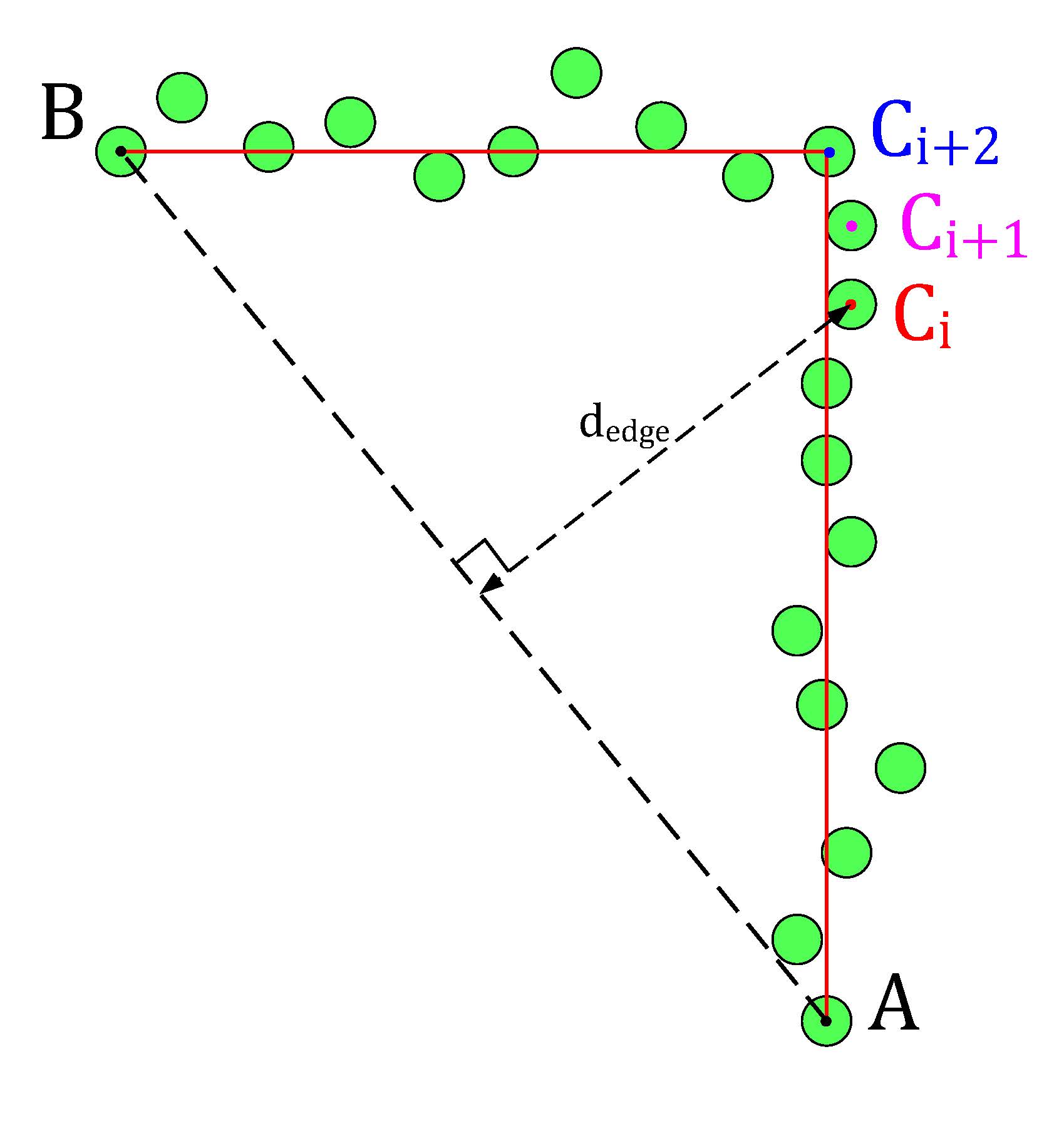
• Edge detection: the line detection algorithm only detects if data points have a large distance relative to each other. The edge detection function detects if the line-segments (which result from the line detection) contain edges. The basic idea of the implemented algorithm can be seen in the figure below. The line segment in that figure has a starting data point A and an end point B. A virtual line, AB, is the drawn from point A to B. Finally the distance from the data points C_i, which lie inside the segment, to the virtual line AB is calculated, d_edge. The largest value d_edge can be considered an edge.

• 

  Line detection algorithm of the PICO robot.

• 

  Edge detection algorithm of the PICO robot.

With the ability to observe and locate walls, gaps can be easily detected. basic idea of this gap detection algorithm is that the robot looks for large distances between subsequent lines. The threshold for this difference can be tuned in order to set the minimum gap size. The world model not only stores the local coordinates of gaps, but it also stores the exit walls. The function gapDetect in the class Perception is responsible for storing both the gaps and exit walls in the world model. The visualization beneath shows the localization of a gap in a room. The bright red circle represents the set-point to which PICO will drive towards. This set-point contains a small adjustable margin which prevents collisions with nearby walls.

Gap detection in custom Escape room

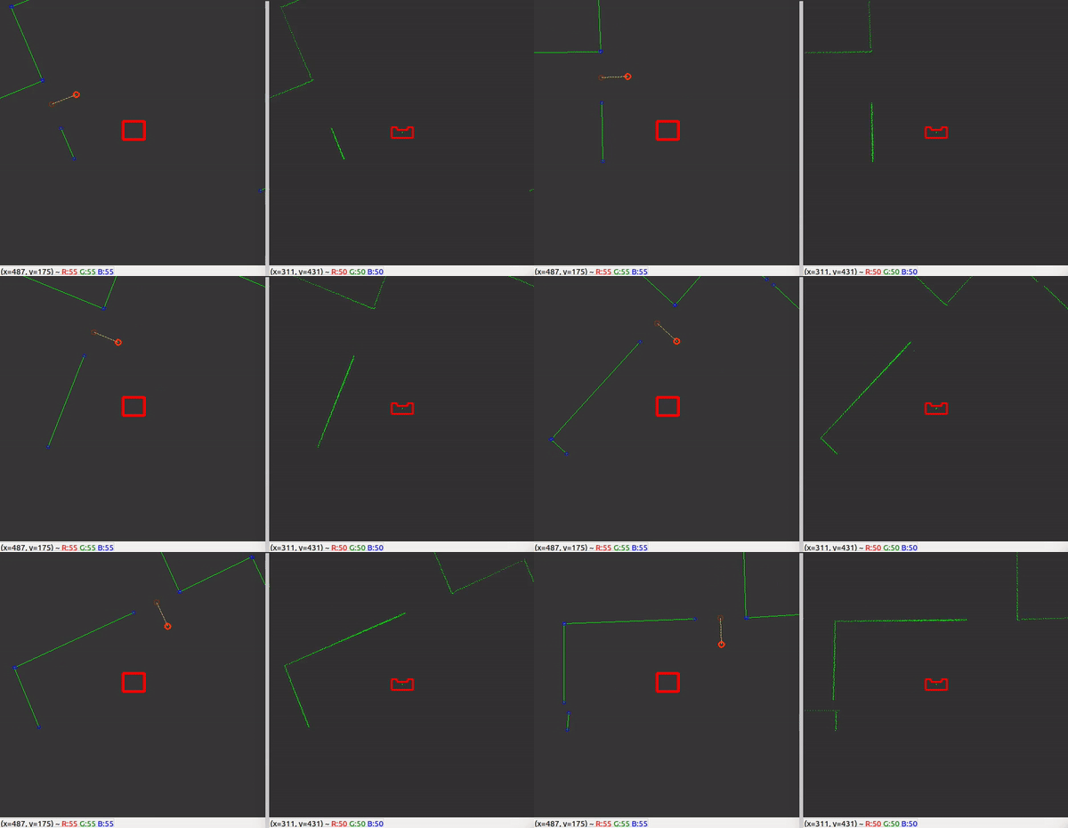
Some additional features were added, which adds robustness to the line/edge and the gap detection:

• Adjustable parameter MIN_LINE_LENGTH which sets the minimum amount of data points for which we can define a line. With this implementation stray data points will not be perceived as lines.
• Adjustable parameter MIN_GAP_SIZE, which sets the minimum gap size. When the gap size between two lines is lower than this value, everything inside that gap is ignored.
• Adjustable parameter GAP_MARGIN, which as previously mentioned adds a margin to the gap set-point.

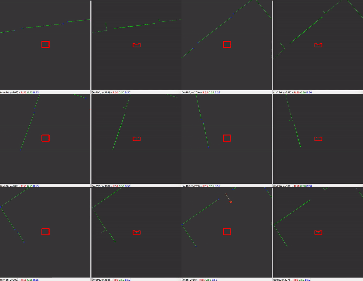
With these features, a rather robust perception component has been developed. The resulting performance can be seen in the recording below. The detected lines and gap have been visualized. Small gaps and lines which are present in this custom map are ignored.

Ignoring small gaps and short lines

World Model

The world in the Escape room challange, stored the following features:

• segments: this member variable in the world model class contains every line segment in a vector. A Line struct has been added which stores the beginning position and end position index and coordinates. The coordinates can be stored with a Vec2 struct.
• gaps: this member variable in the world model class contains the perceived gaps in a vector. A Gap struct has been implemented which stores the gap coordinates (Coords), the gap coordinates including a margin (MCoords) and the gap size.
• exit_walls: this memeber variable contains the 2 exit walls in a vector. These walls are stored as the before mentioned Line struct.

Keep in mind that these features are being renewed constantly during the operation of PICO.

Monitor and strategy

The goal of Monitor is to map the current situation into discrete states using information of the environment. For the escaperoom four different situations are checked, namely whether a wall, a gap, a corner or an exitwall is found in Perception.

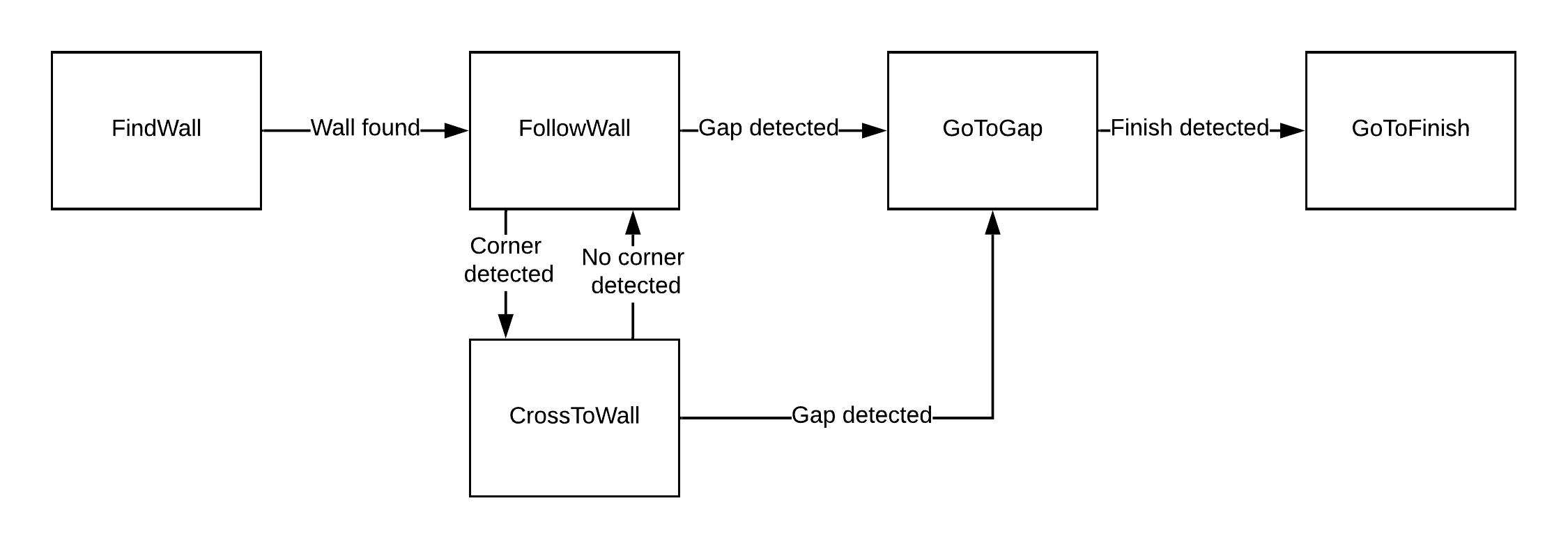
Strategy controls a Finite State Machine, shown in the figure below, that is used to determine which action Control should take. The discrete states from Monitor are used for the guards of this final state machine. When the state machine is in the state FindWall, Control get the objective to move untill a wall is detected. In the state FollowWall Control follows the wall which is the closest to the robot. From FollowWall it can either go to GoToGap, when a gap is detected, or to CrossToWall. In CrossToWall the objective for Control is to follow the wall that is perpendicular to the wall it is currently following. This way the corner is cut-off. When the gap is detected the robot directly goes to this gap and when it recognizes the finish it will drive to the finish.

Finite State Machine used in the escape room challenge.

Control

In control, a main functionality is to drive towards a target. Therefore the function "GoToPoint()" is created. This function allows the robot to drive towards a point in its local coordinates. The input is a vector which defines the point in local coordinates. Reference velocities are send towards the base in order to drive towards this point. Updating this point frequently makes sure that the robot will have very limited drift, as the reference and thus the trajectory will be adjusted. The robot will not drive and only turn when the angle towards the point is too high, this angle is made into a tunable parameter.

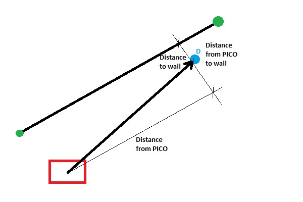
For our strategy, it is necessary that PICO can follow a wall, hence a “FollowWall( )” function is created. The “FollowWall( )” function creates an input point (vector) for the “GoToPoint( )” function. To create this point two parameters are used. One for the distance from the wall to the destination point, and one for the distance from PICO to the destination point. Both are tunable parameters. With the use of some vector calculations this point is created in local coordinates. The benefit of this method is that drift is eliminated, since the point is updated each timestep. Also PICO will approach the wall in a smooth curve and the way this curve looks like is easy tuned by altering the parameters. The following figure presents this approach.

Follow wall algorithm.

Challenge

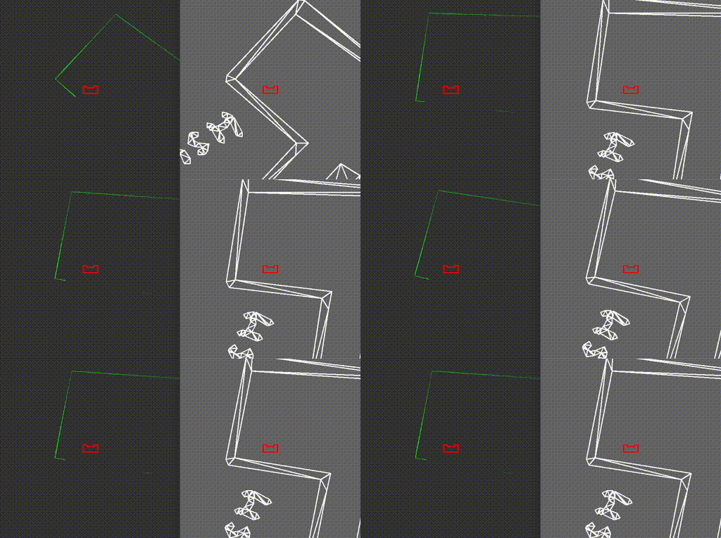
On May 13th the escape room challenge was held, where the task was to exit a simple rectangular room through its one exit without any prior information about the room. We had prepared two branches of code, to allow ourselves to have a backup. With the software described in the previous sections, the first attempt showed behavior which was very close to the video below. Unfortunately, when the robot turned its back towards the wall it should be following, it got stuck in a loop which it could not escape. From the terminal we could read that the robot remained in a single state, called FollowWall. However, its reference direction did constantly change.

Performance during the escape room challenge

The code for the second attempt, which omitted the use of the states GoToGap and GoToFinish, made use of two states only, being FindWall and FollowWall. This meant that the issue we faced in the first attempt was still present in the new code, hence exactly the same behavior was observed.

During the interview, it was proposed by our representative that the issue was a result of the robot turning its back to the wall, meaning that the wall behind it is not entirely visible. In fact, because the robot can not see directly behind, the wall seems to be made out of two parts. During turning, the part of the wall which is closest to the robot is used in the FollowWall function changes, hence the reference point changes position. Then, with the new reference point the robot turns again, making the other section of the wall closest, causing the robot to turn back and enter a loop.

During testing with the room that was provided after the competition, a different root to our problems was concluded. As it turned out, the wall to the rear left of the robot almost vanishes when the robot is turning clockwise and its back is facing the wall, as can be seen in the left video above. This means that this wall no longer qualifies as a wall in the perception algorithm, hence it is not considered as a reference wall anymore. This means that the robot considers the wall to its left as its reference, meaning that it should turn counterclockwise again to start moving parallel to that. At that point, the wall below it passes over the threshold again, triggering once again clockwise movement towards the exit.

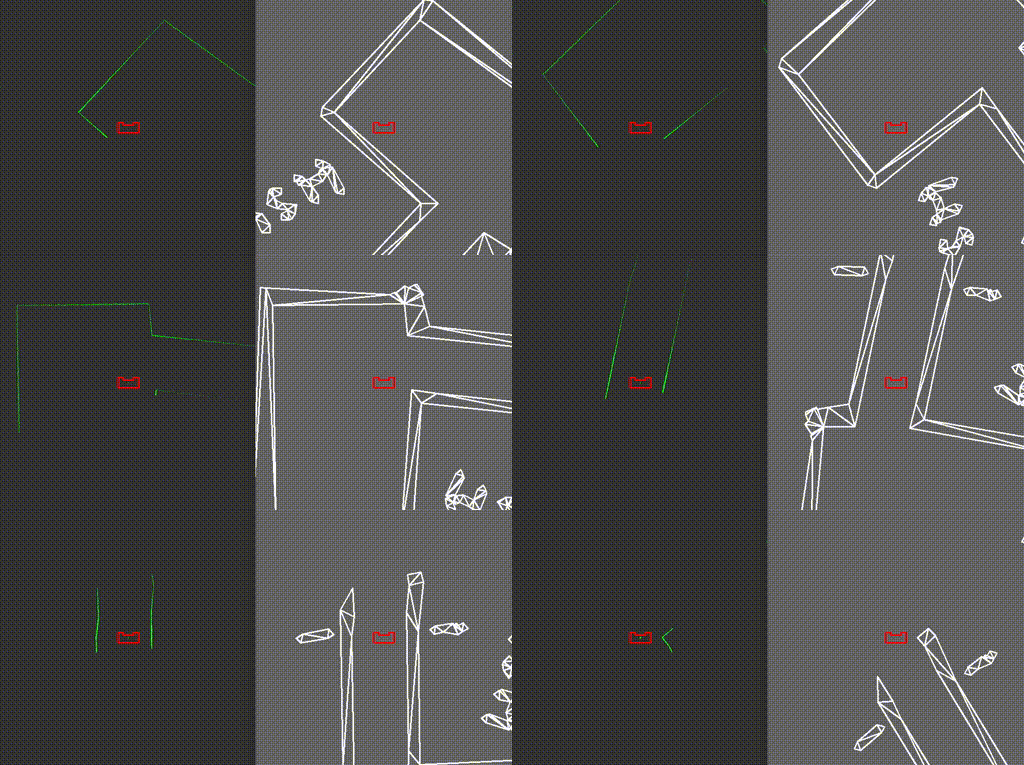
With this new observation about the reason the robot got stuck, which could essentially be reduced to the fact that the wall to be followed passed under the threshold, the first debugging step would be to lower this threshold. Reducing it from 50 to 20 points, allowed the robot to turn clockwise far enough, so that the portion of the wall towards the exit came closest and hence could be followed. This meant that the robot was able to drive towards the exit, and out of the escape room without any other issues, as can be seen in the video below. All in all, it turned out that the validation we had performed before the actual challenge missed this specific situation where the robot was in a corner and had to move more than 90 degrees towards the exit. As a result, we did not tune the threshold on the minimum amount of points in a wall well enough, which was actually the only change required to have the robot finish the escaperoom.

Performance during the escape room challenge after the corrections.

Hospital Challenge

INLEIDING

Information Architecture

In order to finish the hospital challenge, we have first created an information architecture. The basics structure is very related to the escape room challenge. The architecture is created in a logical manner, as it first locates the robot in perception, then stores this data in the world model from which the strategy is determined and the robot is actuated through a control structure. The components within the architecture contain the following components:

• Config. Reader: Is able to parse through JSON-files which contains points, walls and cabinets present within the map; Can also parse through JSON-files containing each waypoint and it neighbors.
• Monitor & Strategy: BLABLABLABLABLABLABLABLABLA!
• Perception: Localizes PICO in the global map using a Monte Carlo particle filter; Detects unknown objects in the global map.
• World Model; Stores the global map and local map; Stores the path list and waypoints link matrix.
• Visualization: Contains plot functions meant for debugging several components; Contains the mission control visualization used for the final challenge.
• Control: BLABLABLABLABLABLABLABLABLABLA!

The following figure shows functions, functionalities and states within each component.

Improved information architecture which has been used for the hospital challenge.

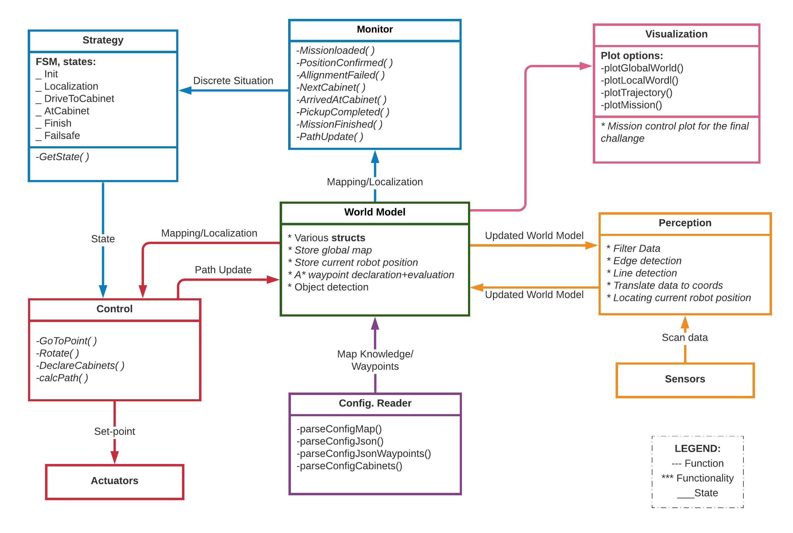
In comparison to the escape room challenge, the information architecture has not changed much. The only difference is the addition of 2 components: the Visualization and the Config. Reader. The visualization became crucial in the debugging phase of several functionalities and components within the software architecture. While the config. reader helped improve the A* path planning and loading in several testing maps. In the following sub-chapters, again the main functionalities of each component will be explained and discussed.

Config. Reader

The config. reader component is a new component added after the escape room challenge. This components can parse through several types of files. For the Hospital challenge, three types of parses have been used:

1. parseConfigJson(): parses throught the supplied JSON file of the hospital map
2. parseConfigJsonWaypoints(): parses throught the waypoints coordinates and neighbors
3. parseConfigCabinets(): parses through the cabinets orientations in the hospital map

Monitor & Strategy

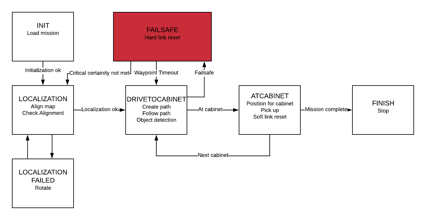
The hospital challenge is tackled with the following Finite State Machine (FSM) which is implemented in strategy. The guards are implemented in monitor.

The first state of PICO is the INIT state. This is the initialization, and here the mission is loaded. When the mission is loaded the initialization is finished and Pico goes into the LOCALIZATION state. When PICO is in the LOCALIZATION state, the localization is performed. When PICO confirms that he knows his position it is checked whether the conditions for correct localization are met. This means that PICO should have used at least three edges for the localization. If this is not the case, or when PICO needs to many iterations to localize, PICO will go to the LOCALIZATION FAILED state. In this state PICO will make a small rotation, after which it goes back into the LOCALIZATION state. When the localization is confirmed, PICO goes to the DRIVETOCABINET state. In this state, a path is calculated and followed. When PICO is following its path, it keeps scanning the environment to continuously in order to confirm its position and to detect objects. When a static object is detected it is checked whether this object blocks a link which is in the path that PICO is currently following. When this is the case, a new path will be calculated, avoiding the link that is blocked by the object. The path PICO is following consists of several waypoints. A timer is set when a waypoint is reached. If PICO does not reach the next waypoint before the timer ends or when the position uncertainty get too high, it will go in to the FAILSAFE. In the FAILSAFE the linkmatrix is reset. Dependent on the reason the FAILSAFE state is reached, it will go back into LOCALIZATION or DRIVETOCABINET. When PICO is close to the cabinet it is heading to in the DRIVETOCABINET state, it goes into the ATCABINET state. In this state PICO alligns with the heading of the cabinet, and performs the pick up. A snapshot of linesegments is made and it is checked whether the cabinet is the last one of the mission, in which case the mission is completed and the FINISH state is reached. If the mission if not completed, the linkmatrix will get a soft reset. This means that only the links that have had a small increase in weight are reset. After this PICO goes back to the DRIVETOCABINET state.

This FSM is taken as a guidance throughout developing the functions.

Perception

The most important task which perception has to complete is the localization of the robot. This is chosen to be done by using a 'Monte Carlo Particle filter'. This is chosen over other techniques as it is not limited to parametric distributions and is relatively simple to implement. Also, it outperforms other non-parametric filters such as the histogramfilter (reference). The LRF is used to recognize features, which is used in the feature-based sensor model. The features considered are convex and concave corners. As the robot is to be positioned within three degrees of freedom, at least three corners are needed for a proper localisation. The position of the robot is updated with odometry data in combination with this PF filter to account for uncertainties such as drift.

Implementation

In the beginning of the hospital challenge, the position and orientation of PICO is unknown. Based on its LRF data, PICO should be able to find its global position and orientation on the provided map. As the map is known, a Monte Carlo particle filter can be used, which is a particle filter algorithm used for robot localization. This algorithm can be summarized by the following pseudo code:

for 1 to NUMBEROFPARTICLES do

  Generate particle with random position and orientation
  Translate the global position of the (known) corners to the local coordinate frame of the particle
  Filter out the corners not within the LRF range of the particle
  Calculate probability by comparing the seen corners of the particle with the corners PICO sees

end

Weighting the probabilities of all the particles to sum up to one
Resample the particles according to weight
Calculate the average of the remaining particles
Calculate the uncertainty by comparing the corners PICO sees with the corners the computed average position should see
Update the range where particles are generated according to this uncertainty

In order to validate the localisation of PICO, a simple test map is made. To also test robustness against unknown objects and object detection, a same test map is made with a object in the right lower corner.

Test map for localisation.

Test map for localisation, with object.

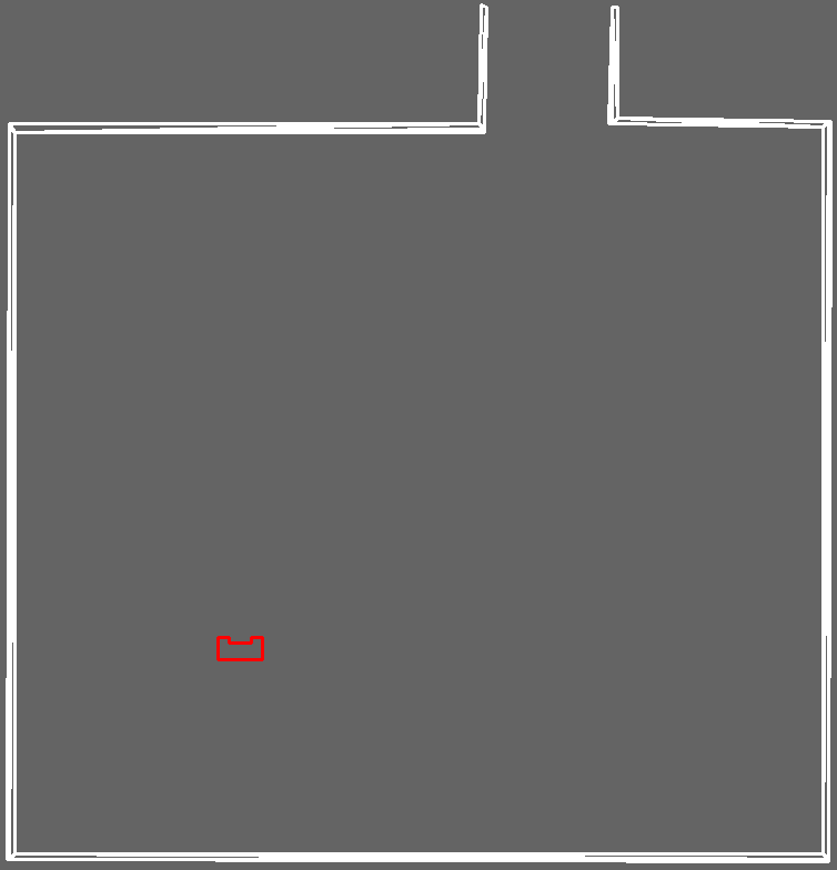
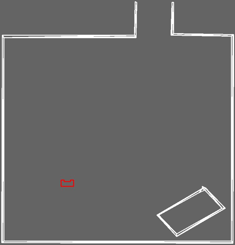
General PF algorithm

Resampling particles with the highest probability.

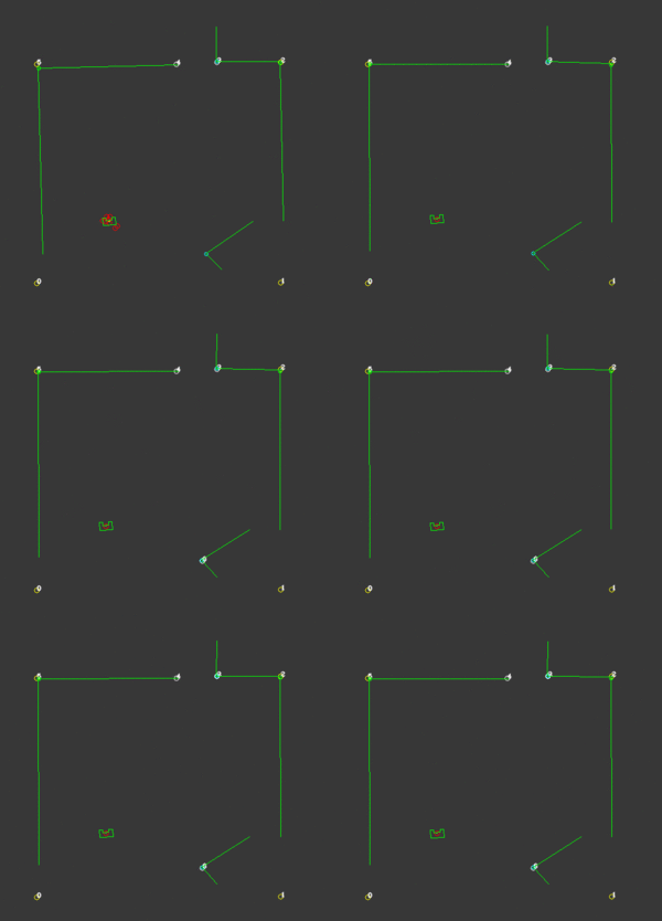
The first step is create particles with random position and orientation. Then, for each particle, what it should see is compared to what PICO ‘sees’ at the moment, from which a probability is calculated. The problem of finding what each particle with random position and orientation on the map should see is the so called ray casting problem. Due to the limited time of this project, it was chosen to solve this problem using a feature-based sensor model. This approach tries to extract a small number of features from high dimensional senor measurements. An advantage of this approach is the enormous reduction of computational complexity [reference to probalistic robotics page 147]. More specific, this approach compares certain features on the map that the particle should see to what PICO sees. As already an edge (or corner) detect function was implemented during the escape room challenge, it was decided to use these corners as features. An alternative would be to use the walls as features. However the difficulty with walls was that they are only partly visible, while the corners are visible or not. In order to assign a better probability to each particle, the edge detect function is updated to distinguish convex and concave corners. After assigning a probability to each particle, they should be resampled according to this new probability distribution. First all the probabilities are weighted, so that the sum of all probabilities equals one. Then from this distribution the particles are resampled. After a few resamples, PICOs position and orientation is the average of the remaining particles. The number of particles generated and the number of resamples can be changed in the configuration and are fine tuned by considering the trade-off between computational load and accuracy of the computed position.

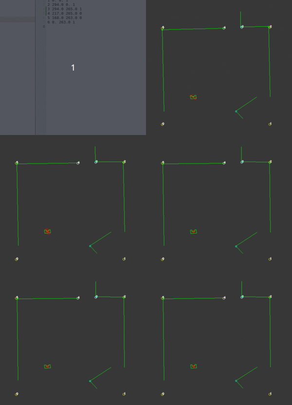
On the right, a visualization of the localisation using the particle filter is shown. It shows how after a few resamples, the correct position of PICO is found. The yellow and white circles represent the convex and concave corners present in this map. The green and blue circles represent the convex and concave corners observed by PICO. The red circles represent the resampled particles.

Converging algorithm

Converging to the right position when initially incorrect.

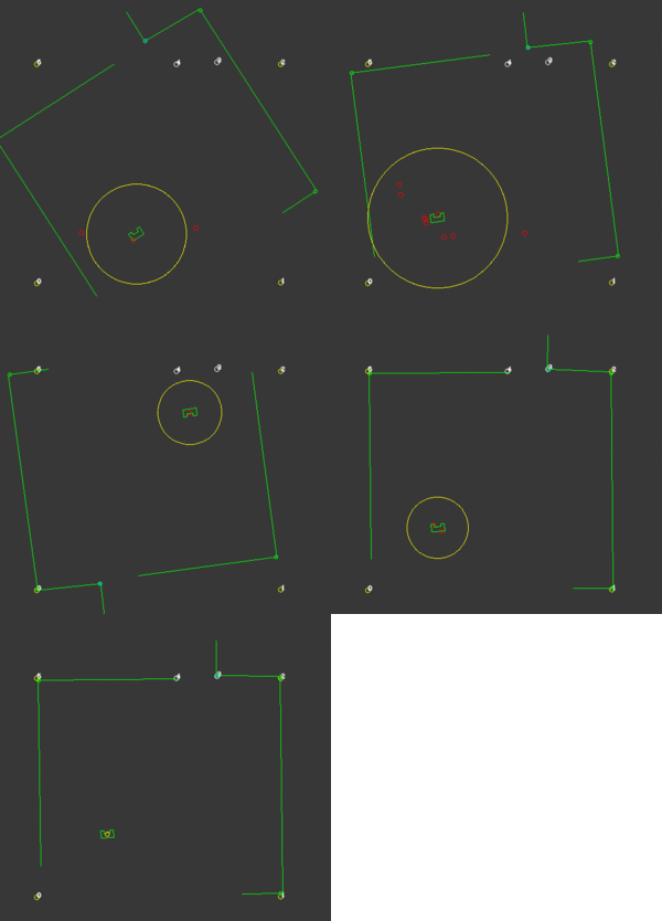
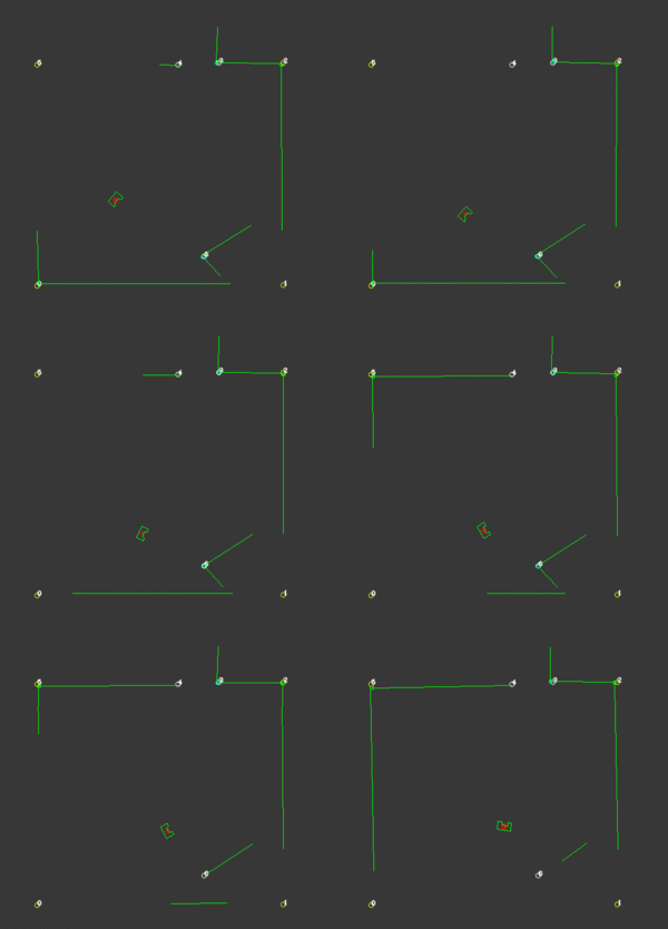
At this position, the local position of the visible corners are translated to the global coordinate frame using the obtained global position of PICO. Then, the global position of these convex and concave corners are compared to their actual (known) global location on the map, by computing the distance between them. This quantity is then used as an uncertainty measure, as this value would be very small if all the seen corners are placed on the right location. This uncertainty measure is first multiplied by a weight and then used to update the range of particles generated around PICOs position when the PF algorithm reruns. This ensures that the global position of PICO always converges to the right position. This weight can be changed in the configuration and is fine tuned by considering how aggressive the PF should react to uncertainty. When a high value is chosen, the computed position converges more quickly to the right position. However this would make the localisation less robust against corners from unknown obstacles.

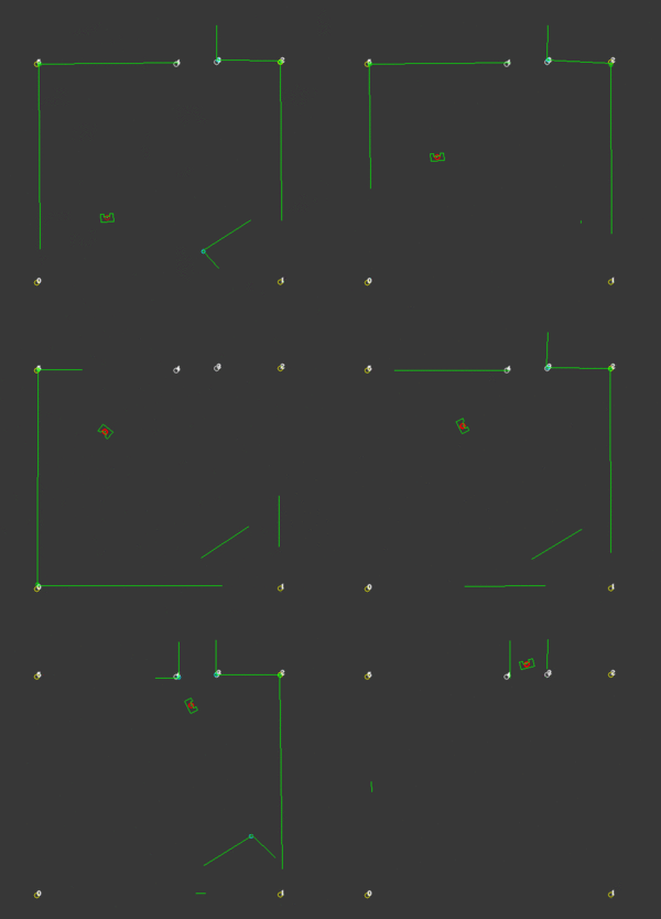
On the right, a visualization is seen of a situation where PICO first initially assesses its position at a wrong location. However due to the uncertainty evaluated after the particle filter, it corrects and converges to the right position. The yellow circle around PICO represents its uncertainty.

Updating using odometry data

Updating location using odometry data.

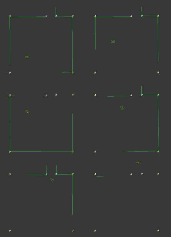
When driving, the position and orientation of PICO is updated with the odometry data. When PICO drifts, the previously described uncertainty measure will increase as the distance between the visible edges and the known edges increases. As a result the range around PICO where particles are generated increases, from which the right position can again be recovered. As PICO sometimes only drifts in a certain direction, the particle range around PICO is made as an ellipse in order to account especially for the drifting direction.

Feature based sensor model (probability function)

(explaining prob function in more depth)

Resampling function

Resampling, graphic representation.

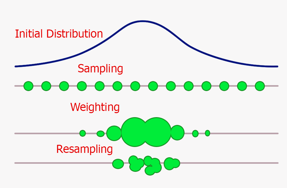
One of the main reasons the particle filter is computationally efficient, is due to the resampling step. It is possible to implement this filter without this step, however this would require a very large amount of particles for obtaining similar accuracy. After assigning each random generated particle with a probability. All probabilities are weighted in order for the total probability to be equal to one. Then, using the same already generated particles are resampled according to this weight. If for example one very accurate particle gets a weighted probability of 50%, means that during resampling this particle will be chosen approximately half of the total number of particles. After resampling, the probability of each particle is recalculated according to the number of times it has been chosen. The particles that have not been chosen are removed. The probability of all the particles are again weighted for the total sum to be equal to one. This resampling step can be done one or several times for each run of the PF algorithm.

Configuration parameters/Conditions on localization/Robustness against unknown edges

(number of resamples, number of particles, weighting uncertainty in distance to new particle range, division of initialization and driving, seeing at least 3 edges, fixed uncertainty when seeing less than 3 corners, how do we cope with unknown corners (obstacles))

Localisation with unknown edge of obstacle. Initialization.

Localisation with unknown edge of obstacle. Driving.

Object detection

Unknown edge detected as an object.

New added edge used for better localisation.

World Model

Visualization

The visualization is being done with the help of the OpenCV library, which is available though ros. The World Model supplies the Visualization component with information, which is translated to OpenCV objects (e.g. cv::Point, cv::Circle, etc.). There exists 3 different plot functions meant for debugging. These are: plotLocalWorld(), plotGlobalWorld(), plotTrajectory(). Each plotting function served the purpose to help debugging a specific part of the code. In the figure below a simplified information architecture has been made. This figure also shows in which part of the code the plotting functions were used to debug. A short de

The locations within the code structure, where the plotting function are meant to help debugging.

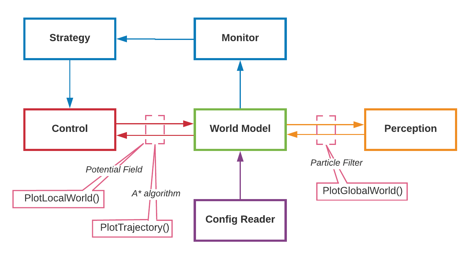
• plotLocalWorld(): which plots the components in the local map: local walls, local edges, PICOs safe-space (as previously shown in the potential field subchapter)
• plotGlobalWorld(): which plots the components in the global map. It plots in red the particles with highest probability. It shows the area (in yellow) in which the particle are being placed. The walls and edges observed via the LRF data can also be seen, this time in global coordinates.
• plotTrajectory(): which plots the trajectory points and links. The weight of each link is also shown in order to test the link breaking mechanism (e.g. when doors are closed in the hospital). The path which is chosen is highlighted, and the current waypoint to which PICO is navigating is highlighted in orange.

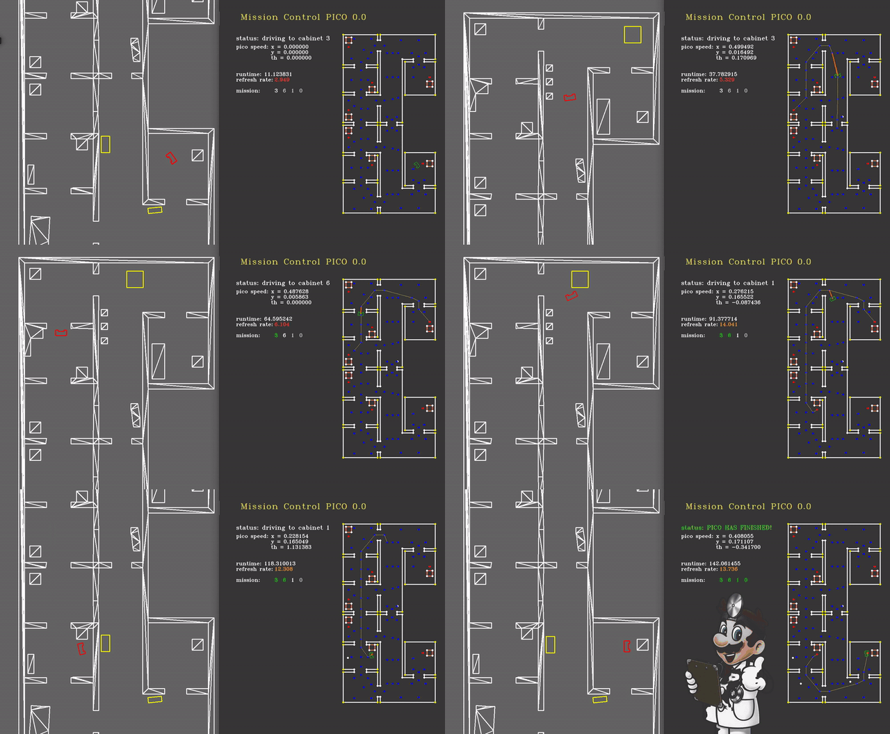
For the hospital challenge an additional plotting function has been written called, plotMission(). This visualization shows the user a nice overview of the mission, including:

• the cabinet to which PICO is driving,
• the speed of PICO in x, y and theta direction,
• the runtime and framerate,
• and the list of cabinets to which PICO is/has driving/driven.

Control

Control has to create a path towards the cabinet and, using the current strategy, drive towards this cabinet. To create a global path, the A* algorithm is used, to avoid hitting objects or cutting corners, a local/sensor-based path planning is used with a potential field algorithm.

Global path planning

In order for the robot to navigate its way through a roughly known area, it benefits from all prior information about the shape, size and dependencies of the different rooms and corridors. One common way of shaping this information in a tangible and concise manner is by gridding the entire space into smaller areas. Consequently, these areas contain information about the presence of nearby walls or objects, allowing for some path to be calculated from any position to any of the predefined targets. Following this path is then a task for a low-level-controller, which compares the position of the robot to the desired position on the path and asymptotically steers the error to zero.

Waypoints

In our case, the choice has been made to import all available data more cleverly. Instead of gridding the entire area into equally sized squares or hexagons, a clever network of waypoints was introduced to capture all the relevant information. These waypoints, which are shown in Figure ??, could be thought of as only those grid areas that are required to traverse the rooms and corridors, instead of all of them. It would not make sense to consider grid areas in a corner the robot is either unable to ever reach, or is very unlikely to be the optimal path. Instead, waypoints would be cleverly defined before and after doors, in the middle of rooms and corridors and near cabinets. Due to the fact that unknown objects may be encountered while driving through the hospital, multiple waypoints are placed around each room, allowing for multiple routes to be taken between them. Moreover, as can be seen in the large vertical corridor in Figure ??, in corridors, multiple waypoints are placed next to each other for redundancy. For both rooms and corridors, the presence of multiple feasible options should be guaranteed, even in the presence of large, possibly dynamical objects. A total of 90 waypoints have been chosen to accurately and efficiently grid the entire hospital layout.

Seven of the waypoints have a special purpose, namely that they represent the positions in front of the cabinets. Specifically, they indicate the position centered in front of the cabinet, at a distance of 0,3 [m] to cause less interference with the repulsive force from the cabinet calculated in the potential field algorithm. These waypoints representing cabinets are strictly not different from the others, but they are accompanied by a file containing information on which waypoints represent which cabinets, and which heading is required to face the cabinet.

Links

Between all waypoints, links can now be introduced, containing information about feasibility and some measure of the cost to follow that link. These links can be thought of as the roads on a real-life roadmap, where the waypoints are intersections and crossroads. Then, an ordinary satellite navigation system is capable of calculating the optimal path from its current position to some desired destination, using only these links and their associated costs. In fact, by adapting the costs of these links online, or in the case of a real-life system using external communication, a highly flexible dynamic map of all relevant travelling options is maintained. This map can then be used to synthesize an optimal path, with optimality in a user-defined sense. In the case of our robot, we have specified in the input file all possible links that originate from each waypoint. Generally, this means that at each waypoint, approximately 3-8 options are available to continue a path, reducing the computational requirements of the optimal path synthesis. Moreover, a simple function was designed to calculate a relevant measure of cost of a link, which we decided to be the Euclidean distance between the two waypoints the link connects. Travel time was also considered instead of distance, however under the mild assumption of an equal velocity over all links, there seemed to be little benefit. This function is used as the initialization of the network of links, as well as the hard reset of all links by the failsafe. The benefit of only considering the pre-defined options for links is that no checks have to be performed by the robot to prevent links from passing through walls.

The resulting network of waypoints and links is visualized in Figure ??, where the links are indicated by the yellow lines. On top of each link, the cost is shown in white, rounded off to an integer. As mentioned above, this cost is basically the only over which is optimized when determining a path from a starting point to a cabinet. Therefore, this cost is the most logical way to dissuade the robot from following certain links. In the situation, for instance, where the robot finds a closed door ahead, it should ‘break’ the link passing through that door by increasing its cost severely. Instead of doing this at the first time a door is observed, the cost of the link through the door is increased rapidly over 10-20 iterations, to prevent noisy measurements from breaking too many links. Each iteration where a link is increased, it is considered whether the current path has become infeasible, after which a new optimal path is calculated. The rapid increase in link costs in the presence of a door and in the presence of a dynamical object are shown in Figure ??, where special attention should be given to the white numbers accompanying the links.

Detecting intersections

Unlike the situation where the network of links is initialized, where use could be made of the pre-defined set of allowed links, a detection is required to find intersections between links and newly found objects. Consider the door of the example mentioned in the previous paragraph, where the door is defined as a line segment between two points. Since we know the exact start and end point of the links as well, we should be able to calculate whether or not the two lines intersect. A first approach, based on linear polynomials of the form y = ax+b falls short in situations where nearly vertical lines are identified, or when the lines do in fact intersect, whereas the line segments do not. Instead, a method was developed based on the definition of a line segment as p_{i,start}+\alpha_i*(p_{i,end}-p_{i,start}), with \alpha_i a number between 0 and 1. Then, two line segments i and j can be equated and a solution for \alpha_i and \alpha_j can be found. Barring some exceptional cases where the line segments are for instance collinear, it can be concluded that an intersection between both line segments only occurs when both 0<=\alpha_i<=1 and 0<=\alpha_j<=1. In our software, this approach was implemented by comparing each link to each known line segment on an object. As described in the object detection chapter of this Wiki, the objects are stored as a set of line segments in global coordinates in the world model, ready to be used for detecting intersections.

The intersections between links and objects is not the only relevant case where intersections should be identified to avoid collisions or the robot getting stuck. Identifying a path, using only waypoints and links, is generally not sufficient, as the robot is not always exactly on a waypoint when a new path is calculated. Therefore, ‘temporary links’ may be introduced, originating from the robot its current position and ending in all waypoints, of which the feasibility is not known a priori. Consequently, the same intersection algorithm can be used to assess feasibility for these temporary links, comparing them to known objects around the robot. In order to ensure that the robot does not want to drive along a link which is too narrow for Pico to follow, a ‘corridor’ of Pico’s width is used for this intersection detection instead. Two additional temporary links are placed on both sides of the direct line segment between the robot and each waypoint, of which collisions are also checked. An example of a situation where this ‘corridor’ is required to avoid a deadlock is shown in Figure ??.

A* algorithm

With this definition and implementation of the waypoints and links, all relevant information for a global path planning algorithm is available. Two simple options come to mind, both with the guarantee that an optimum solution is found, namely the Dijkstra’s and the A* algorithm. They are very similar in the sense that they iteratively extend the most promising path with a new link, all the way until the path to the destination has become the most promising. The difference between the two algorithms lies in the assessment of ‘most promising’. For the Dijkstra’s, the only considered measure for promise is the cost-to-go from the initial position of the robot. This results in an equal spread into all directions of the currently considered paths, resulting in a computationally inefficient solution. However, the Dijkstra’s algorithm is always guaranteed to yield an optimal solutions, if it exists. On the other hand, the A* algorithm not only considers cost-to-go, but also takes into account the cost from the currently considered waypoint to the destination. This yields in a much quicker convergence to the optimal solution, especially in the presence of hundreds or even thousands of links. The exact cost from each waypoint to each destination, however, requires an optimization procedure of its own, quickly losing all benefits from the Dijkstra’s approach. However, it turns out that even a relatively inaccurate guess, often referred to as a heuristic, of the cost from a waypoint to the destination greatly benefits computational speed. In our application, this estimate is simply chosen to be the Euclidean distance, not taking into account walls or other objects. This could have been extended by incorporating some penalty in case the link does intersect a wall, but this did not seem like a large improvement and could have been detrimental for stability of the optimization procedure. The advantage of using the Euclidean distance as the heuristic is that its value is always equal to or lower than the actually achieved cost, which happens to be the requirement for the A* algorithm to be convergent to the optimal solution. Note that this heuristic only needs to be calculated once, since all waypoints and destinations are known beforehand and the Euclidean distance never changes.

With the choice for A* as the solver and the availability of the waypoints, links and heuristic, the actual implementation of the global path planning is rather simple. The first iteration calculates the most promising path from the robot to any waypoint, taking collisions and Pico’s width into account. Next, each new iteration the current most promising path is extended into the most promising direction, while preventing waypoints from being visited twice. This iterative procedure only ends when the current most promising path has arrived at the destination cabinet, after which the route is saved into the world model. Due to the fact that the path remains optimal for any point on the path, as stated by the principle of optimality, it does not need to be re-calculated each time instant. Instead, a new path is only calculated if one of three situations arise, namely a cabinet being reached and a new cabinet awaiting, the aforementioned detection of an object on the current path and the robot entering a failsafe.

Whenever the robot reaches a new cabinet and a new path should be calculated, a soft reset is placed on the cost of all links, meaning that the cost all links which have been briefly blocked by an object are reset back to their original value, being their lengths. This distinguishes between static objects and doors on the one hand, who have cause the links they intersect with to far exceed the soft reset threshold, and noise and dynamic objects on the other hand, which have only been identified briefly and therefore had less effect on the cost of the links. This soft reset ensures that the next calculated path will also be optimal, and not effected by temporary or noisy measurements. When an object is detected on the path, no reset needs to be taken place, as we specifically want the robot to find a new route around the object. Thirdly, when the failsafe is entered and a new path is required to be calculated, depending on the cause of the failsafe a hard reset, forgetting all doors and objects, or a soft reset is performed.

Low level control

In order to closely follow the optimal path stored in the world model, a separate function is developed which is tasked to drive towards a point, which is in our case implemented in the GoToPoint() function.

Local path planning - Potential field

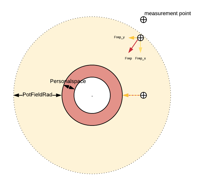
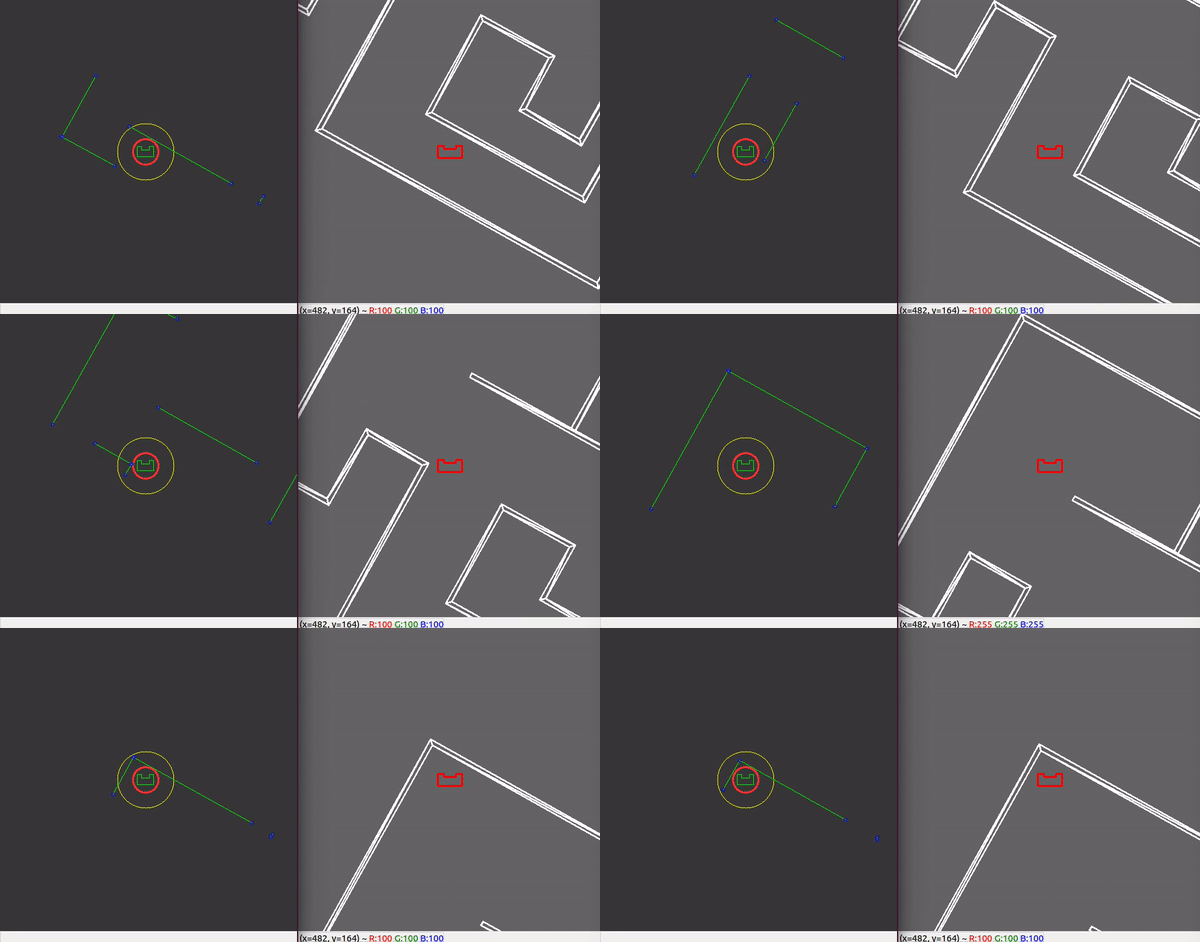
To avoid the robot bumping in to objects, walls or doors, for example with an inaccurate localization, a potential field algorithm is implemented. This is a sensor based strategy, determining in which direction to move. A potential force is created by the sum of an attractive force, coming from the target location, and a repulsive force field, coming from LRF data points around the robot. Every LRF point which is inside the potentialfield radius (a circle from the origin of the robot, with a tunable parameter radius set to 70 centimeters), is taken into account creating a repulsive force vector. The repulsive force of a point scales quadratically depending on the distance from the robot. The repulsive and attractive forces are tuned in such a way that the robot will not come closer to a wall or corner than the 'personalspace' (a circle from the origin of the robot, with a tunable parameter radius set to 10 centimeters plus the half of the width of PICO). A schematic is shown in the Figure below.

• 

Choosing the scaling of the repulsive force (e.g. Quadratic (^2) or ^3), as well as the potential field radius and 'personalspace' were tuned during testing. This combination seemed to have the most smooth and robust results. A known and common problem with the potential field algorithm is possible local minima. However, in combination with the global path planning with a lot of way-points and our strategy, local minima are not expected.

The GIF below shows the robot driving towards a local point straight ahead of the robot, not bumping into any walls.

Driving forward with an active potential field.

Final Presentation

Media:Group 6 hospital challenge FINAL PRESENTATION.pdf

Validation

First, all parts were seperately created and it was confirmed they worked. During this process, different visualizations were made and used to debug the individual components. These were later also used to debug the total workings of the code when all parts were implemented.

During implementation of all components, various problems were faced and resolved. This section will shed light on the most prevalent challenges.

The implementation of all components made it such that the code was not always able to run at the desired 20 Hz, sometimes it could not even reach 10 Hz. This caused problems in for example the potential field, which does not function properly when sensor data is only updated after a long time. Due to a hold of the base reference values, pico could run into walls. By adding clock statements in between functions we were able to identify bottlenecks and make the code somewhat more efficient and faster. In order for pico not to run into walls, the speed in the backup code was adjusted to the refresh rate (only in the backup code, because it is a competition and a visualization running into a wall has no big consequences).

implementing localization together with global path planning, was one of the bigger challenges. When the localization would not be accurate, a lot of links would be broken and the robot would not know where to move next. Soft resets and hard resets of weights in the link matrix was added, as well as a failsafe for localization and path planning.

Challenge

During the final challenge, the robot did not finish. This was due to two small problems.

The first problem was that PICO was close to the cabinet but did not go into the 'atcabinet' state. During testing, this was observed a few times, however, the robot was almost always able to converge its localization and get out of the position it seemed stuck in.

What happened is that the localization was just slightly off. As a result, global planning wanted the robot to move slightly further towards the cabinet. However, the local potential field made sure the robot did not move forward anymore. There are several fixes to this problem: - (Recommended) Adjusting the measure of certainty needed for localization around the cabinet. This could be very accurate and is not invasive on the code. It would be an addition to the strategy. - The potential field could be less strict around the cabinet as well as lowering the speed. This, however, could be risky. - Adjusting the config value which says how far the robot should be in front of the cabinet. This is a very quick fix but it could be that the robot will then be too far from the cabinet. - Local positioning based on sensors when close to the cabinet, this could be very precise and an elegant solution, but would require some new functions.

The second problem was a problem that never occurred before the challenge. We observed PICO wanting to drive to a way-point that was directly behind a wall. It did not drive through the wall due to the potential field. At this point PICO was stuck. There are multiple reasons why this happened and multiple options how it could be fixed.

1. PICO should have observed the wall long before it was close to it, he should have broken the link. The reason that PICO did not show this behaviour is because the path weight is added to by increments and are dependent on the refresh rate. The refresh rate was very low and PICO did not break the link before it was driving towards the way-point behind the wall. This can be resolved by either a higher and stable refresh rate or an adding of weight based on time instead of iterations. (A very fast, however less elegant, way of resolving this is raising the increment parameter in the config file) To show that the breaking of this link is no problem with a higher frame rate, the GIF below is given

Breaking a link after observing the door.

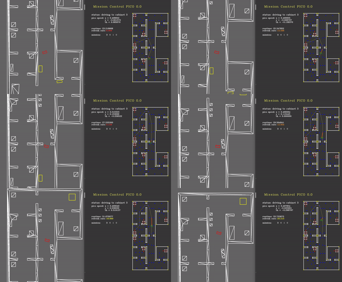
2. The moment that PICO did not reach the way-point behind the wall within 10 seconds, the failsafe was activated. This made all links have the original weight (hard reset) and made PICO create a new path. However, as this new path was via the way-point that he was very close to, he had no time to break the link before he was driving towards the way-point behind the wall again. This infinite loop could be resolved by having the failsafe last a couple of seconds, where PICO is sure of localization and has the time to add weights to the links in the link-matrix, before calculating a new path and following this.

A recommendation following from this for the code as a whole, which would fix and prevent some problems is: The code should either tune its parameters to time, not iterations, OR the code should run at a constant refresh rate which it can always reach. This would require making the code more efficient.

After changing one config parameter, breaking a link more quickly, we tried the hospital challenge again and this is the result:

Hospital challenge.