Embedded Motion Control 2013 Group 1: Difference between revisions
| (132 intermediate revisions by 5 users not shown) | |||
| Line 5: | Line 5: | ||
<tr style="background: #D3D3D3;"> | <tr style="background: #D3D3D3;"> | ||
<td width="150px"><b>Name:</b></td> | <td width="150px"><b>Name:</b></td> | ||
<td width="50px"><b>Abbr:</b></td> | <td width="50px"><b>SVN Abbr:</b></td> | ||
<td width="120px"><b>Student id:</b></td> | <td width="120px"><b>Student id:</b></td> | ||
<td width="170px"><b>Email:</b></td> | <td width="170px"><b>Email:</b></td> | ||
| Line 31: | Line 31: | ||
</tr> | </tr> | ||
<tr> | <tr> | ||
<td>Frank | <td>Frank Hochstenbach</td> | ||
<td>FH</td> | <td>FH</td> | ||
<td>0792390</td> | <td>0792390</td> | ||
| Line 59: | Line 59: | ||
# [[Embedded_Motion_Control_2013_Group_1/Meeting_20130918|Meeting - 2013-09-18]] | # [[Embedded_Motion_Control_2013_Group_1/Meeting_20130918|Meeting - 2013-09-18]] | ||
# [[Embedded_Motion_Control_2013_Group_1/Meeting_20130925|Meeting - 2013-09-25]] | # [[Embedded_Motion_Control_2013_Group_1/Meeting_20130925|Meeting - 2013-09-25]] | ||
# [[Embedded_Motion_Control_2013_Group_1/Meeting_20131016|Meeting - 2013-10-16]] | |||
== | == Planning == | ||
=== Week 1 (2013-09-02 - 2013-09-08) === | === Week 1 (2013-09-02 - 2013-09-08) === | ||
| Line 85: | Line 86: | ||
=== Week 4 (2013-09-23 - 2013-09-29) === | === Week 4 (2013-09-23 - 2013-09-29) === | ||
* Decide which maze solving strategy we are going to use/implement. | * Decide which maze solving strategy we are going to use/implement. | ||
* Test line detection. | |||
=== Week 5 (2013-09-30 - 2013-10-06) === | === Week 5 (2013-09-30 - 2013-10-06) === | ||
* | * Finalize situation node. | ||
* Make line detection more robust. | |||
* Test motion and odometry. | |||
=== Week 6 (2013-10-07 - 2013-10-13) === | === Week 6 (2013-10-07 - 2013-10-13) === | ||
* | * Start working on vision node. | ||
* Test all the nodes working together in the simuatlion. | |||
* Expand the reasoning with the vision. | |||
=== Week 7 (2013-10-14 - 2013-10-20) === | === Week 7 (2013-10-14 - 2013-10-20) === | ||
* | * Make test plan for test on Monday 21-10-13 - Frank | ||
* Add to wiki: Vision, SignalInterpolator, Reasoning, test results 15-10-13 - Multiple people | |||
* Adjust code reasoning so it works with vision - Paul | |||
* Check odometry data for flaws and adjust on wiki - Paul | |||
* Add bag files test to svn - Wouter | |||
* Make presentation - Pieter | |||
* Test vision with test bag files - Niels | |||
* Avoid collision with wall - Frank, Paul & Wouter | |||
* Ros launch file for simulator and real world | |||
=== Week 8 (2013-10-21 - 2013-10-27) === | === Week 8 (2013-10-21 - 2013-10-27) === | ||
* | * Maze challenge | ||
* Final presentation | |||
* Peer to peer review | |||
* Final version wiki | |||
== Progress == | == Progress == | ||
=== Week 1 === | |||
=== Week 2 === | === Week 2 === | ||
=== Week 3 === | |||
* Programmed reasoning for right wall follower. | |||
* Finalized the design of the localization | |||
=== Week 4 === | |||
* Integrated all the nodes into a single launch file. | |||
* Debugged all the nodes and made sure that the output was correct. | |||
* Finalized the design of the situation | |||
=== Week 5 === | |||
* First integral testing are done. | |||
* Made the situation node more robust for false-positives. | |||
=== Week 6 === | |||
* Tested with our software architecture with Pico, unfortunately the bag files we created were to big to be used (for some reason they could not be exported). | |||
* Started with vision, we did choose to use template matching to detect the arrow. | |||
=== Week 7 === | |||
* testing on pico | |||
* debugging issues while testing | |||
=== Week 8 === | |||
Found 3 issues during testing in week 7 | |||
* Reasoner stability; it is a know issue that the situation is unreliable at the beginning of a crossing. A filter was build but is was kicked out for some reason. It will be checked why the filter was deleted. | |||
* Threshold vision; when testing last week it was darker. That's why the thresholds where adjusted. A new bagfile with images is created out of which the new threshold will be determined. | |||
* A known issue in the reasoner; a warning was created which isn't implemented right. | |||
Also the presentation needs updating | |||
== Software architecture == | == Software architecture == | ||
[[File: | [[File:Pico_diagram.png|center|]]<br> | ||
(Note: With the dotted ''B'' line we can either choose, in ''pico_visualization'' to either visualize the message coming from the ''pico_line_detection'', or ''pico_situation'') | |||
=== IO Data structures === | === IO Data structures === | ||
{| border="1" cellpadding="5" cellspacing="0" style=" | {| border="1" cellpadding="5" cellspacing="0" style="border-collapse:collapse;" | ||
| style="background: #D3D3D3;" | '''#''' | |||
| | | style="background: #D3D3D3;" | '''Datatype''' | ||
| | | style="background: #D3D3D3;" | '''Published by''' | ||
| | | style="background: #D3D3D3;" | '''Topic''' | ||
| | | style="background: #D3D3D3;" | '''Freq [Hz]''' | ||
| style=" | | style="background: #D3D3D3;" | '''Description''' | ||
|- | |- | ||
| A | | A | ||
| [http://docs.ros.org/api/sensor_msgs/html/msg/LaserScan.html LaserScan] | | [http://docs.ros.org/api/sensor_msgs/html/msg/LaserScan.html LaserScan.msg] | ||
| Pico | | Pico | ||
| /pico/laser | | /pico/laser | ||
| Laser scan data. For info click [http://docs.ros.org/api/sensor_msgs/html/msg/LaserScan.html here] | | 21 | ||
| Laser scan data. For info click [http://docs.ros.org/api/sensor_msgs/html/msg/LaserScan.html here]. | |||
|- | |- | ||
| B | | B | ||
| [ | | [[#Lines|Lines.msg]] | ||
| pico_line_detector | | pico_line_detector | ||
| /pico/line_detector/lines | | /pico/line_detector/lines | ||
| | | 20 | ||
| Each element of lines is a line which exists out of two points with a x- and y-coordinate in the [http://en.wikipedia.org/wiki/Cartesian_coordinate_system cartesian coordinate system] with Pico being the center e.g. (0,0). The x- and y-axis in centimeters and the x-axis is in front/back of Pico while the y-axis is left/right. Further the coordinate system moves/turns along with Pico. | |||
|- | |- | ||
| C | | C | ||
| [ | | [[#Localization|Localization.msg]] | ||
| | | pico_situation | ||
| /pico/ | | /pico/situation/localization | ||
| | | 20 | ||
| The four floats represent the angular mismatch and respectively the distance to the wall with respect to the front, left and right. | |||
|- | |- | ||
| D | | D | ||
| | | [[#Situation|Situation.msg]] | ||
| pico_situation | |||
| /pico/situation/situation | |||
| 20 | |||
| Each boolean, which represents a situation e.g. opening on the left/right/front, is paired with a float which represents the distance to that opening. | |||
|- | |- | ||
| E | | E | ||
| | | [[#Reasoning|Reasoning.msg]] | ||
| | | pico_reasoning | ||
| | | /pico/reasoning | ||
| | | 20 | ||
| The two floats represent the distance to the next decision point and the angle to turn | |||
|- | |- | ||
| F | | F | ||
| | | [http://docs.ros.org/api/geometry_msgs/html/msg/Twist.html geometry_msgs/Twist] | ||
| | | pico_motion | ||
| | | /pico/cmd_vel | ||
| 20 | |||
| first float is the average angle (in radians) between the 2 lines at the sides of pico. The second is the distance to the left hand detected line, the third is the distance to the right hand detected line | | first float is the average angle (in radians) between the 2 lines at the sides of pico. The second is the distance to the left hand detected line, the third is the distance to the right hand detected line | ||
|- | |- | ||
| G | | G | ||
| | | [[#Vision|Vision.msg]] | ||
| | | pico_vision | ||
| | | /pico/vision | ||
| | | 10 | ||
| Sends out two booleans to tell if either a left or right arrow was detected. | |||
|- | |||
| H | |||
| [http://docs.ros.org/api/sensor_msgs/html/msg/Image.html sensor_msgs/Image.msg] | |||
| Pico | |||
| /pico/camera | |||
| ? | |||
| The topic publishes the image from the fish eye camera from Pico. | |||
|- | |||
| I | |||
| [http://docs.ros.org/api/visualization_msgs/html/msg/MarkerArray.html visualization_msgs/MarkerArray] | |||
| pico_visualization | |||
| /pico/line_detection/visualization | |||
| 5 | |||
| The marker array contains a set of [http://docs.ros.org/api/visualization_msgs/html/msg/Marker.html markers]. A marker can be defined to be a certain type of shape either 2D or 3D. In this case the marker is defined as a 2D line. | |||
|} | |} | ||
==== Pico standard messages ==== | |||
To let the different [http://wiki.ros.org/Nodes nodes] communicate with each other they send [http://wiki.ros.org/Messages messages] to each other. ROS defines already a number of different messages such as the [http://wiki.ros.org/std_msgs standard] and [http://wiki.ros.org/common_msgs common] messages. The first provides a interface for sending standard C++ datatypes such as a integer, float, double, et cetera, the latter defines a set of messages which are widely used by many other ROS packages such as the [http://docs.ros.org/api/sensor_msgs/html/msg/LaserScan.html laser scan] message. To let our nodes communicate with each other we defined a series of messages for ourself. | |||
===== Line ===== | |||
The line message includes two points, p1 and p2, which are defined by the [http://wiki.ros.org/geometry_msgs geometry] messages package. A point can have x-, y- and z-coordinates we however only use the x- and y-coordinate. | |||
geometry_msgs/Point32 p1 | |||
geometry_msgs/Point32 p2 | |||
===== Lines ===== | |||
The lines message is just a array of the Line.msg. Using this messages we can send a array of lines to another node. | |||
Line[] lines | |||
===== Localization ===== | |||
The localization message includes 4 [http://docs.ros.org/api/std_msgs/html/msg/Float32.html float32]'s. Angle holds the angular mismatch of the robot with respect to the wall. The distance_front holds the distance with respect to the front wall if any is detected, in case no front wall is detected a special value is assigned. Respectively distance_left and distance_right are used for the distance w.r.t. wall for the left and right side. | |||
float32 angle | |||
float32 distance_front | |||
float32 distance_left | |||
float32 distance_right | |||
===== Reasoning ===== | |||
The reasoning message includes 2 float32's one to represent the distance to the next decision point, and one to describe the angle to turn. | |||
float32 distance | |||
float32 angle | |||
===== Situation exit ===== | |||
The situation exit message uses a [http://docs.ros.org/api/std_msgs/html/msg/Bool.html boolean] and a float32 to specify if a exit is present and the distance from the robot to that exit. | |||
bool state | |||
float32 distance | |||
===== Situation ===== | |||
Since there are three types of exits the situation message has three variables of the type Situation_exit, described above, for either the front, left and right wall. | |||
Situation_exit front | |||
Situation_exit left | |||
Situation_exit right | |||
===== Encoder ===== | |||
The message tells how much Pico has turned, it increases from 0 degrees to either 90 degrees or 180 degrees. | |||
float32 incAngle | |||
===== Drive ===== | |||
The drive message sends commands to the drive node which actually sends the velocity commands to pico. The message contains two float32, one to specify the velocity forwards and one to represent the velocity by which Pico turns around his axis. | |||
float32 speed_angle | |||
float32 speed_linear | |||
===== Vision ===== | |||
The vision message contains two booleans for if it either detects a arrow pointing to the left, or a arrow pointing to the right. | |||
bool arrow_left | |||
bool arrow_right | |||
=== Line detection === | === Line detection === | ||
The ''pico_line_detection'' node is responsible for detecting lines with the laser scanner data from Pico. The node retrieves the laser data from the topic ''/pico/laser''. The topic has a standard ROS [http://wiki.ros.org/sensor_msgs sensor message | The ''pico_line_detection'' node is responsible for detecting lines with the laser scanner data from Pico. The node retrieves the laser data from the topic ''/pico/laser''. The topic has a standard ROS [http://wiki.ros.org/sensor_msgs sensor] message datatype namely [http://docs.ros.org/api/sensor_msgs/html/msg/LaserScan.html LaserScan]. The datatype includes several variables of interest to us namely; | ||
[[File:Pico_grid.png|thumb|right|Definition of the x- and y-axis of Pico]] | [[File:Pico_grid.png|thumb|right|Definition of the x- and y-axis of Pico ]] | ||
# ''float32 angle_min'' which is the start angle of the scan in radian | # ''float32 angle_min'' which is the start angle of the scan in radian | ||
| Line 182: | Line 325: | ||
==== Hough transform ==== | ==== Hough transform ==== | ||
[[File:Hough_Lines.jpg|thumb|right|Line expressed Cartesian coordinate system with <math>(x,y)\,\!</math> and in Polar coordinate system with <math>(r, \theta)\,\!</math>]] | [[File:Hough_Lines.jpg|thumb|right|Line expressed Cartesian coordinate system with <math>(x,y)\,\!</math> and in Polar coordinate system with <math>(r, \theta)\,\!</math><br/>([http://docs.opencv.org/doc/tutorials/imgproc/imgtrans/hough_lines/hough_lines.html Image source])]] | ||
The Hough transform is a algorithm which is able to extract features from e.g. a image or a set of points. The classical Hough transform is able to detect lines in a image. The generalized Hough transform is able to detect arbitrary shapes e.g. circles, ellipsoids. In our situation we are using the probabilistic Hough line transform. This algorithm is able to detect lines the same as the classical Hough transform as well as begin and end point of a line. | The Hough transform is a algorithm which is able to extract features from e.g. a image or a set of points. The classical Hough transform is able to detect lines in a image. The generalized Hough transform is able to detect arbitrary shapes e.g. circles, ellipsoids. In our situation we are using the probabilistic Hough line transform. This algorithm is able to detect lines the same as the classical Hough transform as well as begin and end point of a line. | ||
| Line 199: | Line 342: | ||
| [[File:Hough_Space_2.jpg|center]] | | [[File:Hough_Space_2.jpg|center]] | ||
|} | |} | ||
<div style="text-align:center">([http://docs.opencv.org/doc/tutorials/imgproc/imgtrans/hough_lines/hough_lines.html Image source])</div> | |||
The three plots intersect in one single point namely <math>(0.925,9.6)\,\!</math> these coordinates are the parameters <math>(\theta,r)\,\!</math> or the line in which <math>(x_{0}, y_{0})\,\!</math>, <math>(x_{1}, y_{1})\,\!</math> and <math>(x_{2}, y_{2})\,\!</math> lay. Now we might conclude from this that at this point there is a line i.e. to find the lines one has to find the points in the Hough space with a number of intersections which is higher then a certain threshold. Finding these points in the Hough space can be computational heavy if not implemented correctly. However there exists very efficient [http://en.wikipedia.org/wiki/Divide_and_conquer_algorithm divide and conquer] algorithms for 2D peak finding e.g. see these [http://courses.csail.mit.edu/6.006/spring11/lectures/lec02.pdf course slides] from MIT. | The three plots intersect in one single point namely <math>(0.925,9.6)\,\!</math> these coordinates are the parameters <math>(\theta,r)\,\!</math> or the line in which <math>(x_{0}, y_{0})\,\!</math>, <math>(x_{1}, y_{1})\,\!</math> and <math>(x_{2}, y_{2})\,\!</math> lay. Now we might conclude from this that at this point there is a line i.e. to find the lines one has to find the points in the Hough space with a number of intersections which is higher then a certain threshold. Finding these points in the Hough space can be computational heavy if not implemented correctly. However there exists very efficient [http://en.wikipedia.org/wiki/Divide_and_conquer_algorithm divide and conquer] algorithms for 2D peak finding e.g. see these [http://courses.csail.mit.edu/6.006/spring11/lectures/lec02.pdf course slides] from MIT. | ||
In pseudocode the HoughTransform looks as follows. | |||
'''algorithm''' HoughTransform '''is''' | '''algorithm''' HoughTransform '''is''' | ||
| Line 208: | Line 352: | ||
'''output:''' Set ''L'' lines with the pair (''r'',''theta'') | '''output:''' Set ''L'' lines with the pair (''r'',''theta'') | ||
define 2D matrix | define 2D matrix ''A'' being the accumelator (houghspace) with size/resolution of ''theta'' and ''r'' | ||
'''for each''' ''row'' '''in''' ''M'' '''do''' | '''for each''' ''row'' '''in''' ''M'' '''do''' | ||
| Line 228: | Line 372: | ||
'''return''' ''L'' | '''return''' ''L'' | ||
==== | ==== Robustness ==== | ||
Sometimes however the algorithm jitters a little e.g. it detects a line and in the next sample with approximatly the same data it fails to detect a line. To make the algorithm more robust against this we implemented three methods from which we can choose. They were implemented at the same time since they were quiet easy to implement in the code and it gave us a option to compare them and decided which method we wanted to use in the end. We collect a multiple set of datapoints of data points after which we use either one of the three methods | |||
# Upsampling, use all of the collected datapoints for line detection. | |||
# [http://en.wikipedia.org/wiki/Moving_average Moving average filter], average the datapoints from the multiple sets, then use the average. | |||
# [http://en.wikipedia.org/wiki/Median_filter Median filter], for corresponding datapoints find the median. | |||
These three very simple approaches reduce the jitter to approximately no jitter at all. It is hard to tell which method gives the best result. However it seemed that the third method is best, this can also be explained because the median filter makes sure that samples that are off are not taken into account while in the moving average filter they are taken into account, since of the averaging. | |||
=== Situation === | |||
The situation node interprets the lines which are being published by the pico_line_detector. First it categorizes each detected line. Then it determines the situation regarding Pico's localization followed by the characterization of the hall way e.g. checking if Pico can turn left, right to a new corridor or can keep moving forward in the same corridor. | |||
==== | ==== Categorization ==== | ||
[ | As explained the situation node first categorizes all the lines which are published by the pico_line_detector. Each line has a type number which tells us something about the line. The type is a [http://en.wikipedia.org/wiki/Mask_%28computing%29 bitmask] field. We use 6 bits to specify a line type: | ||
[[File:Pico_grid_3.png|thumb|right|Definition of the quadrants and the line types.]] | |||
* Q1 - 1 - First quadrant | |||
* Q2 - 2 - Second quadrant | |||
* Q3 - 4 - Third quadrant | |||
* Q4 - 8 - Fourth quadrant | |||
* VE - 16 - Vertical line | |||
* HO - 32 - Horizontal line | |||
=== | The first 4 bits tell us in which quadrant the line lays. The first bit is set if a point of a line belongs to quadrant 1. If the second point also belongs to that same quadrant then nothing changes e.g. the first bit is still set and the other three are still zero. If however the second point belongs to quadrant 2 for example then the second bit is set as such the first and second bit are set and we know that the line overlaps to quadrant 1 and 2. | ||
The last two bits determine if a line is vertical or horizontal (One might wonder why we use two bits but this is to rule out some special cases which may occure e.g. a line which stretches from Q1 to Q3 or similar cases). A line is deemed horizontal if the slope of that line is less then 1, otherwise it is deemed to be a vertical line. | |||
The characteristics Q1,...,HO of the line type have been defined as a enum such that we can easily work with it in our code. Using this technique we can easily determine the type of all the different lines with which we are represented with. Further what comes in handy is that we can store our categorized lines in a [http://en.wikipedia.org/wiki/Associative_array map] with the line type being the key and the line itself the value. Also since we are not interested in the order of the map we even use a [http://en.wikipedia.org/wiki/Hash_table hash map]. This enables us to access elements from the map in [http://en.wikipedia.org/wiki/Time_complexity#Constant_time constant time] while a normal map has a lookup time which is logarithmic to the size of the map. To select a certain line we only have to do [http://en.wikipedia.org/wiki/Mask_%28computing%29#Arguments_to_functions ''hashmap.find(Q1 | Q2 | VE)''], herein ''|'' is a [http://en.wikipedia.org/wiki/Bitwise_operation#OR bitwise-or operation], to select the vertical line which overlaps from Q1 to Q2. | |||
Now it maybe possible that we detect some multiple lines with the same type. When this is the case the line with the largest length over rules the others. | |||
==== Localization ==== | |||
To make sure that the robot does not drive against a wall we need to localize Pico with respect to the walls and give a reference to the motion node regarding it. | |||
As explained the lines from pico_line_detector are categorized. There are 9 line types which are eligible to use for localization of Pico. These are: | |||
# Right side | |||
## Q1 | Q4 | VE | |||
## Q1 | VE | |||
## Q4 | VE | |||
# Left side | |||
## Q2 | Q3 | VE | |||
## Q2 | VE | |||
## Q3 | VE | |||
# Front | |||
## Q1 | Q2 | HO | |||
## Q1 | HO | |||
## Q2 | HO | |||
Now we loop threw the entries of the right side e.g. first check if line type Q1 | Q4 | VE exists then Q1 | VE and then Q4 | VE. If either one of them exists we calculate the distance and the angular mismatch with respect to wall and break out of the loop. We then continue by checking the left side and following up the front side. Further since we only sent out one angle we determine the angle with find the angle with the highest priority e.g. first Q1 | Q4 | VE, then Q2 | Q3 | VE, then Q1 | Q2 | HO, then Q1 | VE, etcetera. In pseudo code it looks like this: | |||
'''algorithm''' localization '''is''' | |||
'''input:''' map ''M'' with (key,value)-(''line_type'',''line'') | |||
'''output:''' A tuple ''msg'' with the elements (''distance_right'',''distance_left'',''distance_front'',''angle'') | |||
define 1D array ''l'' | |||
define 2D array ''t'' | |||
define 2D array ''lineTypes'' with the following elements { { Q1|Q4|VE, Q1|VE, Q4|VE }, | |||
{ Q2|Q3|VE, Q2|VE, Q3|VE }, | |||
{ Q1|Q2|HO, Q1|HO, Q2|HO } } | |||
'''for each''' ''row'' '''in''' ''lineTypes'' '''do''' | |||
'''for each''' ''column'' '''in''' ''lineTypes'' '''do''' | |||
'''if''' key ''lineType'' exists in ''M'' | |||
''l''<sub>(''row'')</sub> ← calculate distance w.r.t. to the wall | |||
''t''<sub>(''row'',''column'')</sub> ← calculate angular mismatch w.r.t. to the wall | |||
stop with looping around the columns and start with the next row. | |||
'''for each''' ''column'' '''in''' ''lineTypes'' '''do''' | |||
'''if''' ''t''<sub>(1,''column'')</sub> is set | |||
''msg''.''angle'' ← ''t''<sub>(1,''column'')</sub> | |||
stop with looping | |||
'''else if''' ''t''<sub>(2,''column'')</sub> is set | |||
''msg''.''angle'' ← ''t''<sub>(2,''column'')</sub> | |||
stop with looping | |||
'''else if''' ''t''<sub>(3,''column'')</sub> is set | |||
''msg''.''angle'' ← ''t''<sub>(3,''column'')</sub> | |||
stop with looping | |||
msg.distance_right ← l<sub>(1)</sub> | |||
msg.distance_left ← l<sub>(2)</sub> | |||
msg.distance_front ← l<sub>(3)</sub> | |||
'''return''' ''msg'' | |||
==== Situation ==== | |||
[[File:Pico_situation.png|right|Situation illustration for the lines Q1|Q2|HO and Q2|Q3|VE.]] | |||
The situation determines using the categorized lines in what kind of situation/state the robot is in. If it is approaching a junction and if yes what kind of junction and what is the distance to that junction. The situation nodes posts its result using the [[#Situation|Situation]] message. | |||
The situation can determine if there is a left, right of front junction by a number of manners. For the front case this is pretty easy. If we don't detect a horizontal line which spans over Q1 and Q2 and if the opening between two possible lines which we might find in Q1 and Q2 is width enough then we can move forward. | |||
For the left and right case it is somewhat more difficult since there are multiple cases which may occure and may indicate that there is a opening to the left respectively the right. We will not discuss all possible situation. Assume that we have the following lines, see figure. | |||
* A, a horizontal line which spans over Q1 and Q2. | |||
* B, a horizontal line which spans over Q2 and Q3. | |||
Now to calculate the width of the opening we need to find the point ''a' ''which is the [http://en.wikipedia.org/wiki/Line-line_intersection intersection] of the lines A and B. After finding this point the width of the opening can be easily calculated by substracting the x-coordinate of point ''b'' from the x-coordinate of point ''a'''. When the width of the opening is larger then the threshold of a opening we continue by calculating the distance at which the robot should turn 90 degrees. This distance is calculated by first determining the [http://en.wikipedia.org/wiki/Line_(geometry)#Cartesian_plane x-intercept] of the line A, following by substracting half of the width of the previously determined opening, i.e. the x-coordinate of point ''c'', by which we obtain the x-coordinate of point ''d'' (which has 0 as the y-coordinate) and thus the distance to the opening of the left. | |||
=== Reasoning === | === Reasoning === | ||
The reasoning module is responsible to solve the maze. For this task the module uses the wall follower algorithm also known as the left-hand or right hand-rule. The principle of wall follower algorithm is based on always following the right wall or always following the left wall. This means that the wall is always on your right hand for example (see picture maze). If the maze is not simply connected (i.e. if the start or endpoints are in the center of the structure or the roads cross over and under each other), than this method will not guarantee that the maze can be solved. For our case there is just one input and output on the outside of the maze, and there are also no loops in it. So the wall follower algorithm is in our case very useful. | |||
[[File:reasoning.jpg|thumb|right|Traversal of a maze using the right hand rule ([http://en.wikipedia.org/wiki/Maze_solving_algorithm Image source])]] | |||
The reasoning module gets information from the previous module about the next decision point. These decision points, are points where a decision should be made for example at crossroads, T-junctions or at the end of a road. At the decision points, the reasoning module determines the direction in which the robot will drive, by using the wall follower algorithm. For example when module gets information about the next decision point, which is a crossroad, then the reasoning module determines that the robot turn 90 degrees at this point so that the robot following the right wall. | |||
There also comes information from the vision module this module, search to arrows on the wall. This arrows refer to the output of the maze and help to solve the maze faster. When there is relevant data from the vision module, this data will overrule the wall follower algorithm. | |||
=== Motion === | === Motion === | ||
== | [[File:Motion.jpg|thumb|right]]<br> | ||
[[File: | |||
The motion node consists of three parts: odometry reader, motion planner and the drive module. Al this parts determine dependent of the input signals (actual position and target position) the drive speed and rotation speed of the Pico robot. | |||
==== Odometry Reader ==== | |||
The odometry reader is used to supply information about the robots rotation when the localization data becomes unreliable. This happens when the robot is executing turn since it is unclear with respect to which wall the robot is orientating itself and can change due to sensor noise. | |||
Using the odometry data from the robot an incremental angle is calculated based on the starting angle and this data. The angle is reset when the robot's turn is completed. | |||
The module implements a zero crossing detection to make sure the output is invariant to the range of the odometry data (<math>-\pi\leq\theta\leq\pi</math>). Using this module the robot can turn more than a full rotation with a valid incremental angle. | |||
==== Motion planner ==== | |||
[[File:Emc01_pico_zones.png|thumb]] | |||
The motion planner has two main goals. The first one is to navigate the robot between the walls dependent of the input information from the localization data published by the situation node.. The second goal is to navigate the robot in the right direction on the decision points. These decision points, are points where a decision should be made, for example at a junction. These decision points, and the decision itself are determined by the reasoning node. | |||
Firstly the navigation to stay between the walls, this navigation provides that the robot stays between the walls and doesn’t hit them. To fullfil this task a simple [http://docs.ros.org/api/control_toolbox/html/classcontrol__toolbox_1_1Pid.html PID controller] is used, using the [http://wiki.ros.org/control_toolbox control toolbox] that ROS provides. The controller controls the angle of Pico with respect to the walls such that it drives parallel with the wall. | |||
[[File:motion_planner_3.jpg|thumb|left]] | |||
When the Pico robot stays in the normal zone it will drives forward and just controls the angle such that the robot stays in the normal zone. If for some reason, for example by friction on the wheels, Pico drives into the warning zone a static error is set on the PID controller such that Pico drives back into the normal zone. If for some reason Pico drives into the danger zone the robot stops, a static error is set on the PID controller such that it relocates itself towards the middle of the wall. Only until this is done it moves forwards again. | |||
[[File:motion_planner_4.jpg|thumb|right]] | |||
Secondly the navigation for the decision points. When the robot is inside the border of the decision point the robot will stop driving (the information about the distance up to the decision point itself comes from the reasoning module). On this moment the navigation to stay between the walls is overruled by the navigation for the decision points. After the robot is stopped the robot will rotate in the correct direction, for example turn -90 degrees. When the rotation is done the navigation to stay between the walls takes over and the robot will drive forward until it is on the next decision point. | |||
==== Drive module ==== | |||
The drive module is meant to realize the desired velocity vector obtained from the motion planner. In the current configuration the desired velocity vector is directly applied to the low level controllers since these controllers causing maximum acceleration. Test on the actual machine must point out whether or not the loss of traction due to this acceleration causes significant faults in the position. | |||
=== Vision === | |||
[[File:Arrow_vision.png|thumb|right|Example of a arrow]] | |||
The last component to be added to the software structure is the Vision module. During the maze contest the vision will help completing the maze faster by recognizing arrows that point in the direction of the exit. These arrows are predefined, in the figure here on the right an example is shown. The arrow has a distinct shape and color that should make it fairly easy to distinguish it from its environment. | |||
The most obvious way of finding the arrow would be by looking for its color, however there are also more red objects in its environment like red chairs and people with red sweaters, this may give false positives. Robustness of the vision is crucial because false positives may cause Pico to move in the wrong direction which costs time and may even prevent it from driving out of the maze at all. Therefore, the vision should only give correct values or nothing at all. Because of this [http://docs.opencv.org/doc/tutorials/imgproc/histograms/template_matching/template_matching.html template matching] was chosen since this is a robust method and most important of all very easy to implement. | |||
==== Template matching ==== | |||
[[File:Img rgb260.png|thumb|right|Image from vision]] | |||
[[File:Temp arrow right.png|thumb|right|Template arrow right]] | |||
The principal of template matching is quite simple. A template is taken of the object that has to be found in a certain image or video. By comparing every part of the image with the template a matrix with values is created. Each value represents the level of similarity, by taking the local minimums or maximums of the matrix (depending on the matching method) the best match can be found. This is how the standard OpenCV library finds the best match. What it does however not take into account is the height of a peak, meaning that it will always find a best match even if there is nothing similar to the template in the image. To solve this a threshold has been implemented in the software which simply compares the highest value with its threshold. For the result to actually represent an arrow its value should be higher then the threshold. It should be noted that this approach only works with non-normalized matching methods, more about this can be read in the next paragraph. | |||
[[File:Example right vision.png|thumb|right|Example arrow recognition]] | |||
As expected the program finds the similarity's between the image and template and draws a rectangle around the found match.<br> | |||
In ROS this would mean that the vision node is now publishing arrow_left = false, arrow_right = true. | |||
==== Matching method ==== | |||
There are 6 different matching methods in the standard OpenCV matching template function. Or to be more exact, there are 3 different methods and each of them is either with or without normalization. The different methods are shown below: | |||
# SQDIFF: <math>R(x,y) = \sum_{x',y'} \left( T(x',y') - I(x + x',y + y')\right)^2</math> | |||
# CCORR: <math>R(x,y) = \sum_{x',y'} \left( T(x',y') - I(x + x',y + y')\right)</math> | |||
# CCOEFF: <math>R(x,y) = \sum_{x',y'} \left( T'(x',y') - I(x + x',y + y')\right)</math> | |||
Herein <math>T'(x',y') = T(x',y') - 1/(w\cdot h) \cdot \sum_{x'',y''} T(x'',y'')</math> | |||
Like said in the previous paragraph, we will not be using the normalized version simply because this causes the program to always find a best match. The method used in the vision software is method 3, CCOEFF, after several simulations and experiments it seems that this method gave the best results. In these formulas the R = result, T = template and I = image. | |||
== Tests == | |||
=== Videos === | |||
The following video's show some simulation tests. | |||
<table border="1" cellpadding="5" cellspacing="0" style="text-align:center;width:100%;border-collapse:collapse;"> | |||
<tr style="background: #D3D3D3;"> | |||
<td><b>Line detection</b></td> | |||
<td><b>Forwards</b></td> | |||
<td><b>Left junction</b></td> | |||
</tr> | |||
<tr> | |||
<td>[[File:Ecm01,_pico_line_detection_-_YouTube.png|200px|center|link=http://www.youtube.com/watch?v=UxnpiemdOHA]]</td> | |||
<td>[[File:Emc01_left.png|200px|center|link=http://www.youtube.com/watch?v=vkDZmVWkMoA]]</td> | |||
<td>[[File:Emc01_left.png|200px|center|link=http://www.youtube.com/watch?v=vkDZmVWkMoA]]</td> | |||
</tr> | |||
<tr style="background: #D3D3D3;"> | |||
<td><b>Right junction</b></td> | |||
<td><b>T junction</b></td> | |||
<td><b>Junction</b></td> | |||
</tr> | |||
<tr> | |||
<td>[[File:Emc01_right.png|200px|center|link=http://www.youtube.com/watch?v=_6YAAs4ZzLo]]</td> | |||
<td>[[File:T-junction.png|200px|center|link=http://www.youtube.com/watch?v=ksmEOcurOYw]]</td> | |||
<td>[[File:Emc01_junction.png|200px|center|link=http://www.youtube.com/watch?v=F6h9LjuJp28]]</td> | |||
</tr> | |||
<tr style="background: #D3D3D3;"> | |||
<td><b>Maze 1</b></td> | |||
<td><b>Maze 2 [http://en.wikipedia.org/wiki/File:Maze01-02.png]</b></td> | |||
<td><b>Maze 3</b></td> | |||
</tr> | |||
<tr> | |||
<td>[[File:Emc01_maze1.png|200px|center|link=http://www.youtube.com/watch?v=Ww2nXZpd5pA]]</td> | |||
<td>[[File:Emc01_maze2.png|200px|center|link=http://www.youtube.com/watch?v=hFybb-t9OBw]]</td> | |||
<td>[[File:Emc01_maze1.png|200px|center|link=http://www.youtube.com/watch?v=5TCOQrK78fQ]]</td> | |||
</tr> | |||
<tr style="background: #D3D3D3;"> | |||
<td><b>Left arrow detection</b></td> | |||
<td><b>Right arrow detection</b></td> | |||
<td><b></b></td> | |||
</tr> | |||
<tr> | |||
<td>[[File:Emc01_arrow_left.png|200px|center|link=http://www.youtube.com/watch?v=SEz2dfgrR5U]]</td> | |||
<td>[[File:Emc01_arrow_right.png|200px|center|link=http://www.youtube.com/watch?v=kayPCPGZXFA]]</td> | |||
<td></td> | |||
</tr> | |||
</table> | |||
=== Week 6: 2013-10-11 === | |||
====Test parameters:==== | |||
We tested with two corridors of width 750 mm and 1000 mm, further we logged the following data. | |||
'''Standard pico topics''': | |||
/pico/camera | |||
/pico/laser | |||
/pico/odom | |||
/tf | |||
/pico/joint_states | |||
'''Our topics''': | |||
/pico/situation/situation | |||
/pico/situation/localization | |||
/pico/line_detection/lines | |||
/pico/line_detection/lines_filtered | |||
/pico/signalInterpolator | |||
/pico/MotionPlanner | |||
====Test results:==== | |||
Motion | |||
* After turning start using localization data in order to keep driving straight | |||
* Start using localization data (width corridor) to determine safety margin distance from wall | |||
* Turning angle is to large, more than 90 degrees | |||
* Margin turn before wall increased, robot kept hitting wall when turning 180 degrees | |||
Localization | |||
* Keep publishing data at all times | |||
=== Week 7: 2013-10-14 === | |||
We tested with two corridors of width 750 mm, further we logged the following data. | |||
'''Standard pico topics''': | |||
/pico/camera | |||
/pico/laser | |||
/pico/odom | |||
/tf | |||
/pico/joint_states | |||
'''Our topics''': | |||
/pico/situation/situation | |||
/pico/situation/localization | |||
/pico/line_detection/lines | |||
/pico/line_detection/lines_filtered | |||
/pico/local_planner/motion | |||
/pico/local_planner/drive | |||
/pico/local_planner/encoder | |||
====Test results:==== | |||
Line detection: | |||
* From looking to the line visualization in rviz the line detection works correctly. | |||
Localization: | |||
* The localization seems to work correctly. We concluded this since the motion works correctly, which bases its output on the localization data. | |||
Situation: | |||
* Sometimes the situation seems to see a corridor to the left where there isn't a corridor to the left. This causes the reasoning to make a false assesment of the situation. | |||
Vision: | |||
* Correctly detects arrows. | |||
Reasoning: | |||
* Bases its conclusion on the data of the situation and seems to work correctly. Also in combination of the vision node it works correctly. | |||
Motion: | |||
* The motion seems to work correctly. The robot keeps driving parallel threw the walls. If the robot is in the danger zone it stops and adjusts it angle. If it is in the warning zone it just adjusts its angle. | |||
=== Week 8: 2013-10-21 === | |||
==== Test document: ==== | |||
For this final test a tight test schedule, [[File:Test_21_10_2013.pdf|thumb|center|]], was created to make sure we are prepared for anything. | |||
====Test results:==== | |||
Line detection: | |||
* Works correctly. | |||
Localization: | |||
* Works correctly. | |||
Situation: | |||
* Still sometimes determines a false situation but most of the times, 99%, it works correctly. | |||
Vision: | |||
* Works correctly. | |||
Reasoning: | |||
* Works correctly. | |||
Motion: | |||
* Works correctly. | |||
====Presentation:==== | |||
[[File:Presentation_v2.pdf|Presentation_v2.pdf]]<br> | |||
== The final challenge == | |||
The challenge was almost completed but failed because of two reasons: | |||
* Vision didn't work because due to the fact that the launch file on the laptop was for a unknown reason not up to date. | |||
* In the tests and simulations we used deeper corridors and more space between the junctions. That is probably why at the end of the maze, Pico made the wrong the decision by going left instead of right. | |||
== | == References == | ||
* Information about maze solving: http://en.wikipedia.org/wiki/Maze_solving_algorithm | * Information about maze solving: http://en.wikipedia.org/wiki/Maze_solving_algorithm | ||
* | * Java applet about Hough transform http://www.rob.cs.tu-bs.de/content/04-teaching/06-interactive/HNF.html | ||
* OpenCV Hough transform tutorial http://docs.opencv.org/doc/tutorials/imgproc/imgtrans/hough_lines/hough_lines.html | * OpenCV Hough transform tutorial http://docs.opencv.org/doc/tutorials/imgproc/imgtrans/hough_lines/hough_lines.html | ||
* OpenCV template matching http://docs.opencv.org/doc/tutorials/imgproc/histograms/template_matching/template_matching.html | |||
</div> | </div> | ||
Latest revision as of 21:53, 27 October 2013
Group Info
| Name: | SVN Abbr: | Student id: | Email: |
| Groupmembers (email all) | |||
| Paul Raijmakers | PR | 0792801 | p.a.raijmakers@student.tue.nl |
| Pieter Aerts | PA | 0821027 | p.j.m.aerts@student.tue.nl |
| Wouter Geelen | WG | 0744855 | w.geelen@student.tue.nl |
| Frank Hochstenbach | FH | 0792390 | f.g.h.hochstenbach@student.tue.nl |
| Niels Koenraad | NK | 0825990 | n.j.g.koenraad@student.tue.nl |
| Tutor | |||
| Jos Elfring | n.a. | n.a. | j.elfring@tue.nl |
Meetings
- Meeting - 2013-09-04
- Meeting - 2013-09-11
- Meeting - 2013-09-18
- Meeting - 2013-09-25
- Meeting - 2013-10-16
Planning
Week 1 (2013-09-02 - 2013-09-08)
- Installing Ubuntu 12.04
- Installing ROS Fuerte
- Following tutorials on C++ and ROS.
- Setup SVN
Week 2 (2013-09-09 - 2013-09-15)
- Discuss about splitting up the team by 2 groups (2,3) or 3 groups (2,2,1) to whom tasks can be appointed to.
- Create 2D map using the laser scanner.
- Start working on trying to detect walls with laser scanner.
- Start working on position control of Jazz (within walls i.e. riding straight ahead, turning i.e. 90 degrees).
- Start thinking about what kind of strategies we can use/implement to solve the maze (see usefull links).
Week 3 (2013-09-16 - 2013-09-22)
- Start work on trying to detect openings in walls.
- Start working on code for corridor competition.
- Continue thinking about maze solving strategy.
Week 4 (2013-09-23 - 2013-09-29)
- Decide which maze solving strategy we are going to use/implement.
- Test line detection.
Week 5 (2013-09-30 - 2013-10-06)
- Finalize situation node.
- Make line detection more robust.
- Test motion and odometry.
Week 6 (2013-10-07 - 2013-10-13)
- Start working on vision node.
- Test all the nodes working together in the simuatlion.
- Expand the reasoning with the vision.
Week 7 (2013-10-14 - 2013-10-20)
- Make test plan for test on Monday 21-10-13 - Frank
- Add to wiki: Vision, SignalInterpolator, Reasoning, test results 15-10-13 - Multiple people
- Adjust code reasoning so it works with vision - Paul
- Check odometry data for flaws and adjust on wiki - Paul
- Add bag files test to svn - Wouter
- Make presentation - Pieter
- Test vision with test bag files - Niels
- Avoid collision with wall - Frank, Paul & Wouter
- Ros launch file for simulator and real world
Week 8 (2013-10-21 - 2013-10-27)
- Maze challenge
- Final presentation
- Peer to peer review
- Final version wiki
Progress
Week 1
Week 2
Week 3
- Programmed reasoning for right wall follower.
- Finalized the design of the localization
Week 4
- Integrated all the nodes into a single launch file.
- Debugged all the nodes and made sure that the output was correct.
- Finalized the design of the situation
Week 5
- First integral testing are done.
- Made the situation node more robust for false-positives.
Week 6
- Tested with our software architecture with Pico, unfortunately the bag files we created were to big to be used (for some reason they could not be exported).
- Started with vision, we did choose to use template matching to detect the arrow.
Week 7
- testing on pico
- debugging issues while testing
Week 8
Found 3 issues during testing in week 7
- Reasoner stability; it is a know issue that the situation is unreliable at the beginning of a crossing. A filter was build but is was kicked out for some reason. It will be checked why the filter was deleted.
- Threshold vision; when testing last week it was darker. That's why the thresholds where adjusted. A new bagfile with images is created out of which the new threshold will be determined.
- A known issue in the reasoner; a warning was created which isn't implemented right.
Also the presentation needs updating
Software architecture
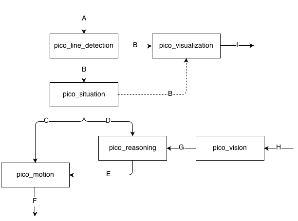
(Note: With the dotted B line we can either choose, in pico_visualization to either visualize the message coming from the pico_line_detection, or pico_situation)
IO Data structures
| # | Datatype | Published by | Topic | Freq [Hz] | Description |
| A | LaserScan.msg | Pico | /pico/laser | 21 | Laser scan data. For info click here. |
| B | Lines.msg | pico_line_detector | /pico/line_detector/lines | 20 | Each element of lines is a line which exists out of two points with a x- and y-coordinate in the cartesian coordinate system with Pico being the center e.g. (0,0). The x- and y-axis in centimeters and the x-axis is in front/back of Pico while the y-axis is left/right. Further the coordinate system moves/turns along with Pico. |
| C | Localization.msg | pico_situation | /pico/situation/localization | 20 | The four floats represent the angular mismatch and respectively the distance to the wall with respect to the front, left and right. |
| D | Situation.msg | pico_situation | /pico/situation/situation | 20 | Each boolean, which represents a situation e.g. opening on the left/right/front, is paired with a float which represents the distance to that opening. |
| E | Reasoning.msg | pico_reasoning | /pico/reasoning | 20 | The two floats represent the distance to the next decision point and the angle to turn |
| F | geometry_msgs/Twist | pico_motion | /pico/cmd_vel | 20 | first float is the average angle (in radians) between the 2 lines at the sides of pico. The second is the distance to the left hand detected line, the third is the distance to the right hand detected line |
| G | Vision.msg | pico_vision | /pico/vision | 10 | Sends out two booleans to tell if either a left or right arrow was detected. |
| H | sensor_msgs/Image.msg | Pico | /pico/camera | ? | The topic publishes the image from the fish eye camera from Pico. |
| I | visualization_msgs/MarkerArray | pico_visualization | /pico/line_detection/visualization | 5 | The marker array contains a set of markers. A marker can be defined to be a certain type of shape either 2D or 3D. In this case the marker is defined as a 2D line. |
Pico standard messages
To let the different nodes communicate with each other they send messages to each other. ROS defines already a number of different messages such as the standard and common messages. The first provides a interface for sending standard C++ datatypes such as a integer, float, double, et cetera, the latter defines a set of messages which are widely used by many other ROS packages such as the laser scan message. To let our nodes communicate with each other we defined a series of messages for ourself.
Line
The line message includes two points, p1 and p2, which are defined by the geometry messages package. A point can have x-, y- and z-coordinates we however only use the x- and y-coordinate.
   geometry_msgs/Point32 p1
   geometry_msgs/Point32 p2
Lines
The lines message is just a array of the Line.msg. Using this messages we can send a array of lines to another node.
Line[] lines
Localization
The localization message includes 4 float32's. Angle holds the angular mismatch of the robot with respect to the wall. The distance_front holds the distance with respect to the front wall if any is detected, in case no front wall is detected a special value is assigned. Respectively distance_left and distance_right are used for the distance w.r.t. wall for the left and right side.
   float32 angle
   float32 distance_front
   float32 distance_left
   float32 distance_right
Reasoning
The reasoning message includes 2 float32's one to represent the distance to the next decision point, and one to describe the angle to turn.
   float32 distance
   float32 angle
Situation exit
The situation exit message uses a boolean and a float32 to specify if a exit is present and the distance from the robot to that exit.
   bool state
   float32 distance
Situation
Since there are three types of exits the situation message has three variables of the type Situation_exit, described above, for either the front, left and right wall.
   Situation_exit front
   Situation_exit left
   Situation_exit right
Encoder
The message tells how much Pico has turned, it increases from 0 degrees to either 90 degrees or 180 degrees.
float32 incAngle
Drive
The drive message sends commands to the drive node which actually sends the velocity commands to pico. The message contains two float32, one to specify the velocity forwards and one to represent the velocity by which Pico turns around his axis.
   float32 speed_angle
   float32 speed_linear
Vision
The vision message contains two booleans for if it either detects a arrow pointing to the left, or a arrow pointing to the right.
   bool arrow_left
   bool arrow_right
Line detection
The pico_line_detection node is responsible for detecting lines with the laser scanner data from Pico. The node retrieves the laser data from the topic /pico/laser. The topic has a standard ROS sensor message datatype namely LaserScan. The datatype includes several variables of interest to us namely;

- float32 angle_min which is the start angle of the scan in radian
- float32 angle_max the end angle of the scan in radian
- float32 angle_increment the angular distance between measurements in radian
- float32[] ranges a array with every element being a range, in meters, for a measurement
Using the above data we can apply the probabilistic Hough line transform to detect lines. The detected lines are then published to the topic /pico/line_detector/lines.
Each line is represented by 2 points in the Cartesian coordinate system which is in centimeters. In the coordinate system Pico is located in the center i.e. at (0,0) and the world (coordinate system) moves along with Pico. The x-axis is defined to be front to back while the y-axis is defined to right to left.
Hough transform
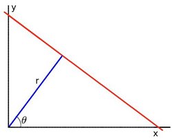
(Image source)
The Hough transform is a algorithm which is able to extract features from e.g. a image or a set of points. The classical Hough transform is able to detect lines in a image. The generalized Hough transform is able to detect arbitrary shapes e.g. circles, ellipsoids. In our situation we are using the probabilistic Hough line transform. This algorithm is able to detect lines the same as the classical Hough transform as well as begin and end point of a line.
How it works. Lines can either be represented in the Cartesian coordinates or Polair coordinates. In the first they are represented in [math]\displaystyle{ y = ax + b\,\! }[/math], with [math]\displaystyle{ a\,\! }[/math] being the slope and [math]\displaystyle{ b\,\! }[/math] being the crossing in the y-axis of the line. Lines can however also be represented in Polair coordinates namely;
[math]\displaystyle{ y = \left(-{\cos\theta\over\sin\theta}\right)x + \left({r\over{\sin\theta}}\right) }[/math]
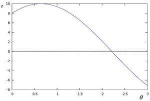
which can be rearranged to [math]\displaystyle{ r = x \cos \theta+y\sin \theta\,\! }[/math]. Now in general for each point [math]\displaystyle{ (x_i, y_i)\,\! }[/math], we can define a set of lines that goes through that point i.e. [math]\displaystyle{ r({\theta}) = x_i \cos \theta + y_i \sin \theta\,\! }[/math]. Hence the pair [math]\displaystyle{ (r,\theta)\,\! }[/math] represents each line that passes by [math]\displaystyle{ (x_i, y_i)\,\! }[/math]. The set of lines for a given point [math]\displaystyle{ (x_i, y_i)\,\! }[/math] can be plotted in the so called Hough space with [math]\displaystyle{ \theta\,\! }[/math] being the x-axis and [math]\displaystyle{ r\,\! }[/math] being the y-axis. For example the Hough space for the point [math]\displaystyle{ (x,y) \in \{(8,6)\} }[/math] looks as the image below on the left. The Hough space for the points [math]\displaystyle{ (x,y) \in \{(9,4),(12,3),(8,6)\} }[/math] looks as the image on the right.
 |
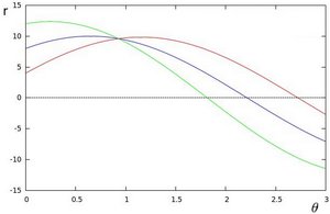 |
The three plots intersect in one single point namely [math]\displaystyle{ (0.925,9.6)\,\! }[/math] these coordinates are the parameters [math]\displaystyle{ (\theta,r)\,\! }[/math] or the line in which [math]\displaystyle{ (x_{0}, y_{0})\,\! }[/math], [math]\displaystyle{ (x_{1}, y_{1})\,\! }[/math] and [math]\displaystyle{ (x_{2}, y_{2})\,\! }[/math] lay. Now we might conclude from this that at this point there is a line i.e. to find the lines one has to find the points in the Hough space with a number of intersections which is higher then a certain threshold. Finding these points in the Hough space can be computational heavy if not implemented correctly. However there exists very efficient divide and conquer algorithms for 2D peak finding e.g. see these course slides from MIT.
In pseudocode the HoughTransform looks as follows.
algorithm HoughTransform is
    input: 2D matrix M
    output: Set L lines with the pair (r,theta)

    define 2D matrix A being the accumelator (houghspace) with size/resolution of theta and r

    for each row in M do
        for each column in M do
            if M(row,column) above threshold
                for each theta in (0,180) do
                    r ← row * cos(theta) + column * sin(theta)
                    increase A(theta,r)

    look at boundary, the center row and the center column of A
    p ← the global maximum within

    if p is a peak do
        add pair (row,column) to L
    else
        find larger neighbour
        recurse in quadrant

    return L
Robustness
Sometimes however the algorithm jitters a little e.g. it detects a line and in the next sample with approximatly the same data it fails to detect a line. To make the algorithm more robust against this we implemented three methods from which we can choose. They were implemented at the same time since they were quiet easy to implement in the code and it gave us a option to compare them and decided which method we wanted to use in the end. We collect a multiple set of datapoints of data points after which we use either one of the three methods
- Upsampling, use all of the collected datapoints for line detection.
- Moving average filter, average the datapoints from the multiple sets, then use the average.
- Median filter, for corresponding datapoints find the median.
These three very simple approaches reduce the jitter to approximately no jitter at all. It is hard to tell which method gives the best result. However it seemed that the third method is best, this can also be explained because the median filter makes sure that samples that are off are not taken into account while in the moving average filter they are taken into account, since of the averaging.
Situation
The situation node interprets the lines which are being published by the pico_line_detector. First it categorizes each detected line. Then it determines the situation regarding Pico's localization followed by the characterization of the hall way e.g. checking if Pico can turn left, right to a new corridor or can keep moving forward in the same corridor.
Categorization
As explained the situation node first categorizes all the lines which are published by the pico_line_detector. Each line has a type number which tells us something about the line. The type is a bitmask field. We use 6 bits to specify a line type:
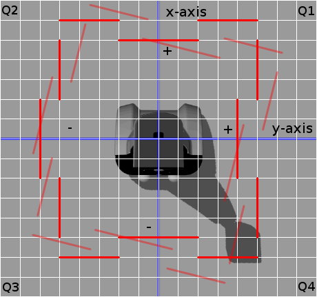
- Q1 - 1 - First quadrant
- Q2 - 2 - Second quadrant
- Q3 - 4 - Third quadrant
- Q4 - 8 - Fourth quadrant
- VE - 16 - Vertical line
- HO - 32 - Horizontal line
The first 4 bits tell us in which quadrant the line lays. The first bit is set if a point of a line belongs to quadrant 1. If the second point also belongs to that same quadrant then nothing changes e.g. the first bit is still set and the other three are still zero. If however the second point belongs to quadrant 2 for example then the second bit is set as such the first and second bit are set and we know that the line overlaps to quadrant 1 and 2.
The last two bits determine if a line is vertical or horizontal (One might wonder why we use two bits but this is to rule out some special cases which may occure e.g. a line which stretches from Q1 to Q3 or similar cases). A line is deemed horizontal if the slope of that line is less then 1, otherwise it is deemed to be a vertical line.
The characteristics Q1,...,HO of the line type have been defined as a enum such that we can easily work with it in our code. Using this technique we can easily determine the type of all the different lines with which we are represented with. Further what comes in handy is that we can store our categorized lines in a map with the line type being the key and the line itself the value. Also since we are not interested in the order of the map we even use a hash map. This enables us to access elements from the map in constant time while a normal map has a lookup time which is logarithmic to the size of the map. To select a certain line we only have to do hashmap.find(Q1 | Q2 | VE), herein | is a bitwise-or operation, to select the vertical line which overlaps from Q1 to Q2.
Now it maybe possible that we detect some multiple lines with the same type. When this is the case the line with the largest length over rules the others.
Localization
To make sure that the robot does not drive against a wall we need to localize Pico with respect to the walls and give a reference to the motion node regarding it.
As explained the lines from pico_line_detector are categorized. There are 9 line types which are eligible to use for localization of Pico. These are:
- Right side
- Q1 | Q4 | VE
- Q1 | VE
- Q4 | VE
- Left side
- Q2 | Q3 | VE
- Q2 | VE
- Q3 | VE
- Front
- Q1 | Q2 | HO
- Q1 | HO
- Q2 | HO
Now we loop threw the entries of the right side e.g. first check if line type Q1 | Q4 | VE exists then Q1 | VE and then Q4 | VE. If either one of them exists we calculate the distance and the angular mismatch with respect to wall and break out of the loop. We then continue by checking the left side and following up the front side. Further since we only sent out one angle we determine the angle with find the angle with the highest priority e.g. first Q1 | Q4 | VE, then Q2 | Q3 | VE, then Q1 | Q2 | HO, then Q1 | VE, etcetera. In pseudo code it looks like this:
algorithm localization is
    input: map M with (key,value)-(line_type,line)
    output: A tuple msg with the elements (distance_right,distance_left,distance_front,angle)

    define 1D array l
    define 2D array t
    define 2D array lineTypes with the following elements { { Q1|Q4|VE, Q1|VE, Q4|VE },
                                                            { Q2|Q3|VE, Q2|VE, Q3|VE },
                                                            { Q1|Q2|HO, Q1|HO, Q2|HO } }

    for each row in lineTypes do
        for each column in lineTypes do
            if key lineType exists in M
                l(row) ← calculate distance w.r.t. to the wall
                t(row,column) ← calculate angular mismatch w.r.t. to the wall
                stop with looping around the columns and start with the next row.

    for each column in lineTypes do
         if t(1,column) is set
             msg.angle ← t(1,column)
             stop with looping
         else if t(2,column) is set
             msg.angle ← t(2,column)
             stop with looping
         else if t(3,column) is set
             msg.angle ← t(3,column)
             stop with looping

    msg.distance_right ← l(1)
    msg.distance_left  ← l(2)
    msg.distance_front ← l(3)

    return msg
Situation
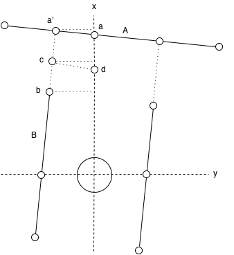
The situation determines using the categorized lines in what kind of situation/state the robot is in. If it is approaching a junction and if yes what kind of junction and what is the distance to that junction. The situation nodes posts its result using the Situation message.
The situation can determine if there is a left, right of front junction by a number of manners. For the front case this is pretty easy. If we don't detect a horizontal line which spans over Q1 and Q2 and if the opening between two possible lines which we might find in Q1 and Q2 is width enough then we can move forward.
For the left and right case it is somewhat more difficult since there are multiple cases which may occure and may indicate that there is a opening to the left respectively the right. We will not discuss all possible situation. Assume that we have the following lines, see figure.
- A, a horizontal line which spans over Q1 and Q2.
- B, a horizontal line which spans over Q2 and Q3.
Now to calculate the width of the opening we need to find the point a' which is the intersection of the lines A and B. After finding this point the width of the opening can be easily calculated by substracting the x-coordinate of point b from the x-coordinate of point a'. When the width of the opening is larger then the threshold of a opening we continue by calculating the distance at which the robot should turn 90 degrees. This distance is calculated by first determining the x-intercept of the line A, following by substracting half of the width of the previously determined opening, i.e. the x-coordinate of point c, by which we obtain the x-coordinate of point d (which has 0 as the y-coordinate) and thus the distance to the opening of the left.
Reasoning
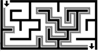
The reasoning module is responsible to solve the maze. For this task the module uses the wall follower algorithm also known as the left-hand or right hand-rule. The principle of wall follower algorithm is based on always following the right wall or always following the left wall. This means that the wall is always on your right hand for example (see picture maze). If the maze is not simply connected (i.e. if the start or endpoints are in the center of the structure or the roads cross over and under each other), than this method will not guarantee that the maze can be solved. For our case there is just one input and output on the outside of the maze, and there are also no loops in it. So the wall follower algorithm is in our case very useful.
The reasoning module gets information from the previous module about the next decision point. These decision points, are points where a decision should be made for example at crossroads, T-junctions or at the end of a road. At the decision points, the reasoning module determines the direction in which the robot will drive, by using the wall follower algorithm. For example when module gets information about the next decision point, which is a crossroad, then the reasoning module determines that the robot turn 90 degrees at this point so that the robot following the right wall. There also comes information from the vision module this module, search to arrows on the wall. This arrows refer to the output of the maze and help to solve the maze faster. When there is relevant data from the vision module, this data will overrule the wall follower algorithm.
Motion
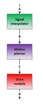
The motion node consists of three parts: odometry reader, motion planner and the drive module. Al this parts determine dependent of the input signals (actual position and target position) the drive speed and rotation speed of the Pico robot.
Odometry Reader
The odometry reader is used to supply information about the robots rotation when the localization data becomes unreliable. This happens when the robot is executing turn since it is unclear with respect to which wall the robot is orientating itself and can change due to sensor noise.
Using the odometry data from the robot an incremental angle is calculated based on the starting angle and this data. The angle is reset when the robot's turn is completed.
The module implements a zero crossing detection to make sure the output is invariant to the range of the odometry data ([math]\displaystyle{ -\pi\leq\theta\leq\pi }[/math]). Using this module the robot can turn more than a full rotation with a valid incremental angle.
Motion planner
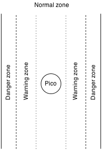
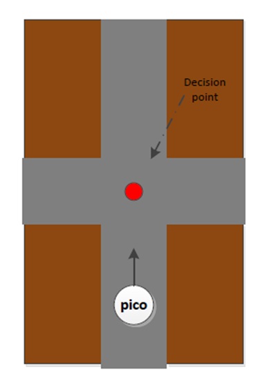
The motion planner has two main goals. The first one is to navigate the robot between the walls dependent of the input information from the localization data published by the situation node.. The second goal is to navigate the robot in the right direction on the decision points. These decision points, are points where a decision should be made, for example at a junction. These decision points, and the decision itself are determined by the reasoning node.
Firstly the navigation to stay between the walls, this navigation provides that the robot stays between the walls and doesn’t hit them. To fullfil this task a simple PID controller is used, using the control toolbox that ROS provides. The controller controls the angle of Pico with respect to the walls such that it drives parallel with the wall.
When the Pico robot stays in the normal zone it will drives forward and just controls the angle such that the robot stays in the normal zone. If for some reason, for example by friction on the wheels, Pico drives into the warning zone a static error is set on the PID controller such that Pico drives back into the normal zone. If for some reason Pico drives into the danger zone the robot stops, a static error is set on the PID controller such that it relocates itself towards the middle of the wall. Only until this is done it moves forwards again.
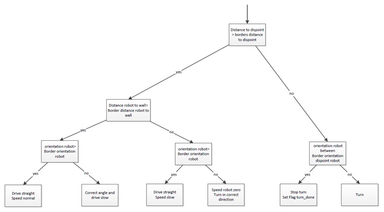
Secondly the navigation for the decision points. When the robot is inside the border of the decision point the robot will stop driving (the information about the distance up to the decision point itself comes from the reasoning module). On this moment the navigation to stay between the walls is overruled by the navigation for the decision points. After the robot is stopped the robot will rotate in the correct direction, for example turn -90 degrees. When the rotation is done the navigation to stay between the walls takes over and the robot will drive forward until it is on the next decision point.
Drive module
The drive module is meant to realize the desired velocity vector obtained from the motion planner. In the current configuration the desired velocity vector is directly applied to the low level controllers since these controllers causing maximum acceleration. Test on the actual machine must point out whether or not the loss of traction due to this acceleration causes significant faults in the position.
Vision

The last component to be added to the software structure is the Vision module. During the maze contest the vision will help completing the maze faster by recognizing arrows that point in the direction of the exit. These arrows are predefined, in the figure here on the right an example is shown. The arrow has a distinct shape and color that should make it fairly easy to distinguish it from its environment.
The most obvious way of finding the arrow would be by looking for its color, however there are also more red objects in its environment like red chairs and people with red sweaters, this may give false positives. Robustness of the vision is crucial because false positives may cause Pico to move in the wrong direction which costs time and may even prevent it from driving out of the maze at all. Therefore, the vision should only give correct values or nothing at all. Because of this template matching was chosen since this is a robust method and most important of all very easy to implement.
Template matching
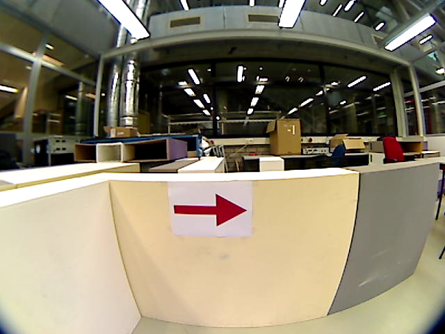

The principal of template matching is quite simple. A template is taken of the object that has to be found in a certain image or video. By comparing every part of the image with the template a matrix with values is created. Each value represents the level of similarity, by taking the local minimums or maximums of the matrix (depending on the matching method) the best match can be found. This is how the standard OpenCV library finds the best match. What it does however not take into account is the height of a peak, meaning that it will always find a best match even if there is nothing similar to the template in the image. To solve this a threshold has been implemented in the software which simply compares the highest value with its threshold. For the result to actually represent an arrow its value should be higher then the threshold. It should be noted that this approach only works with non-normalized matching methods, more about this can be read in the next paragraph.
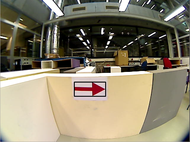
As expected the program finds the similarity's between the image and template and draws a rectangle around the found match.
In ROS this would mean that the vision node is now publishing arrow_left = false, arrow_right = true.
Matching method
There are 6 different matching methods in the standard OpenCV matching template function. Or to be more exact, there are 3 different methods and each of them is either with or without normalization. The different methods are shown below:
- SQDIFF: [math]\displaystyle{ R(x,y) = \sum_{x',y'} \left( T(x',y') - I(x + x',y + y')\right)^2 }[/math]
- CCORR: [math]\displaystyle{ R(x,y) = \sum_{x',y'} \left( T(x',y') - I(x + x',y + y')\right) }[/math]
- CCOEFF: [math]\displaystyle{ R(x,y) = \sum_{x',y'} \left( T'(x',y') - I(x + x',y + y')\right) }[/math]
Herein [math]\displaystyle{ T'(x',y') = T(x',y') - 1/(w\cdot h) \cdot \sum_{x'',y''} T(x'',y'') }[/math]
Like said in the previous paragraph, we will not be using the normalized version simply because this causes the program to always find a best match. The method used in the vision software is method 3, CCOEFF, after several simulations and experiments it seems that this method gave the best results. In these formulas the R = result, T = template and I = image.
Tests
Videos
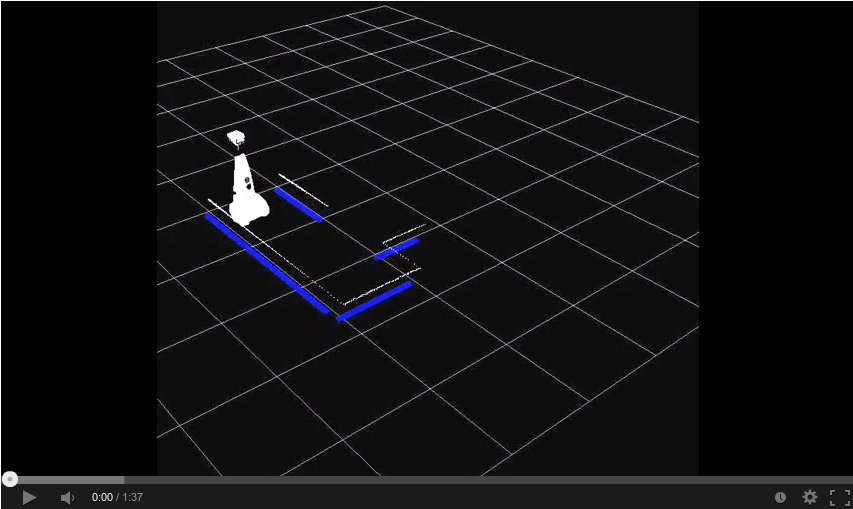
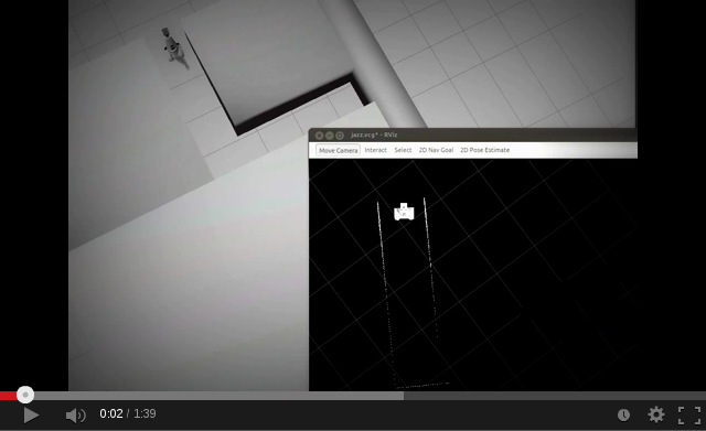
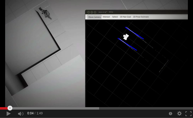
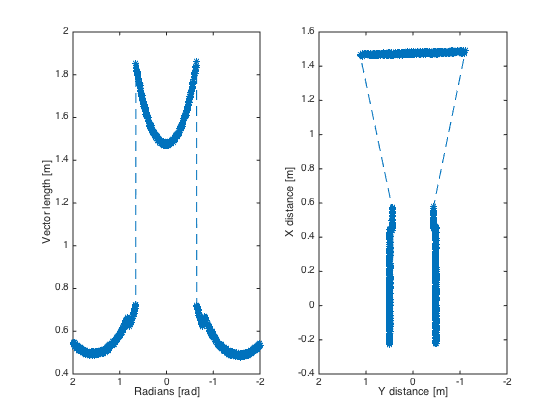
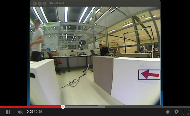
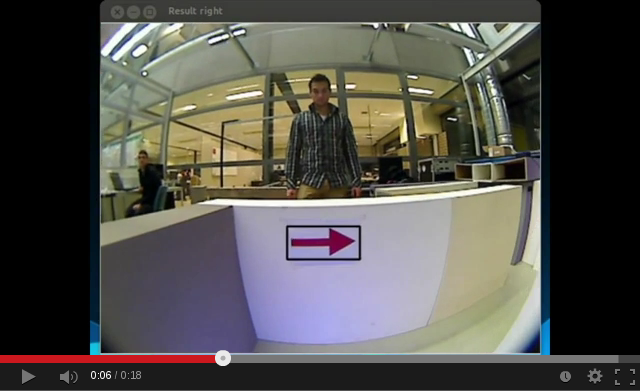
The following video's show some simulation tests.
| Line detection | Forwards | Left junction |
 |
 |
 |
| Right junction | T junction | Junction |
 |
 |
 |
| Maze 1 | Maze 2 [1] | Maze 3 |
 |
 |
 |
| Left arrow detection | Right arrow detection | |
 |
 |
Week 6: 2013-10-11
Test parameters:
We tested with two corridors of width 750 mm and 1000 mm, further we logged the following data.
           Standard pico topics:
           /pico/camera
           /pico/laser
           /pico/odom
           /tf
           /pico/joint_states
           Our topics:
           /pico/situation/situation
           /pico/situation/localization
           /pico/line_detection/lines
           /pico/line_detection/lines_filtered
           /pico/signalInterpolator
           /pico/MotionPlanner
Test results:
Motion
- After turning start using localization data in order to keep driving straight
- Start using localization data (width corridor) to determine safety margin distance from wall
- Turning angle is to large, more than 90 degrees
- Margin turn before wall increased, robot kept hitting wall when turning 180 degrees
Localization
- Keep publishing data at all times
Week 7: 2013-10-14
We tested with two corridors of width 750 mm, further we logged the following data.
           Standard pico topics:
           /pico/camera
           /pico/laser
           /pico/odom
           /tf
           /pico/joint_states
           Our topics:
           /pico/situation/situation
           /pico/situation/localization
           /pico/line_detection/lines
           /pico/line_detection/lines_filtered
           /pico/local_planner/motion
           /pico/local_planner/drive
           /pico/local_planner/encoder
Test results:
Line detection:
- From looking to the line visualization in rviz the line detection works correctly.
Localization:
- The localization seems to work correctly. We concluded this since the motion works correctly, which bases its output on the localization data.
Situation:
- Sometimes the situation seems to see a corridor to the left where there isn't a corridor to the left. This causes the reasoning to make a false assesment of the situation.
Vision:
- Correctly detects arrows.
Reasoning:
- Bases its conclusion on the data of the situation and seems to work correctly. Also in combination of the vision node it works correctly.
Motion:
- The motion seems to work correctly. The robot keeps driving parallel threw the walls. If the robot is in the danger zone it stops and adjusts it angle. If it is in the warning zone it just adjusts its angle.
Week 8: 2013-10-21
Test document:
For this final test a tight test schedule, File:Test 21 10 2013.pdf, was created to make sure we are prepared for anything.
Test results:
Line detection:
- Works correctly.
Localization:
- Works correctly.
Situation:
- Still sometimes determines a false situation but most of the times, 99%, it works correctly.
Vision:
- Works correctly.
Reasoning:
- Works correctly.
Motion:
- Works correctly.
Presentation:
The final challenge
The challenge was almost completed but failed because of two reasons:
- Vision didn't work because due to the fact that the launch file on the laptop was for a unknown reason not up to date.
- In the tests and simulations we used deeper corridors and more space between the junctions. That is probably why at the end of the maze, Pico made the wrong the decision by going left instead of right.
References
- Information about maze solving: http://en.wikipedia.org/wiki/Maze_solving_algorithm
- Java applet about Hough transform http://www.rob.cs.tu-bs.de/content/04-teaching/06-interactive/HNF.html
- OpenCV Hough transform tutorial http://docs.opencv.org/doc/tutorials/imgproc/imgtrans/hough_lines/hough_lines.html
- OpenCV template matching http://docs.opencv.org/doc/tutorials/imgproc/histograms/template_matching/template_matching.html