Embedded Motion Control 2017 Group 6: Difference between revisions
| (150 intermediate revisions by 6 users not shown) | |||
| Line 1: | Line 1: | ||
=='''About the | =='''About the Group'''== | ||
{| border="1" | {| border="1" | ||
| Line 23: | Line 23: | ||
=='''Introduction'''== | =='''Introduction'''== | ||
[[File:Gostai-Jazz-500x500.jpg|thumb|left|Robots | [[File:Gostai-Jazz-500x500.jpg|thumb|left|Robots TACO and PICO]] | ||
The most memorable part of the course Embedded Motion Control is the 'A-MAZE-ING PICO' challenge, in which software is designed for and implemented into autonomous robots. These autonomous robots, called | The most memorable part of the course Embedded Motion Control is the 'A-MAZE-ING PICO' challenge, in which software is designed for and implemented into autonomous robots. These autonomous robots, called PICO and TACO, should then be to able to solve a maze with the software in a real-life environment. A maze can contain loops, dead ends, open spaces and doors that automatically open and close. | ||
PICO will be provided with a basic software layer to carry out primary functions, such as communication and movement. However, to succesfully complete the 'A-MAZE-ING PICO' challenge it is required to design a robust [[#Software Architecture|software architecture]] for the changing environment. Before the software architecture will be realized in C++ it is desired to first decide about the [[#Software Practicalities|software practicalities]]. After some programming several of the [[#Software Subsystems|software subsystems]] will be put to the test in an intermediate challenge. During this challenge, called the [[#Corridor Competition|corridor competition]], PICO must move through a corridor and take the first exit. With the results of the corridor competition and all its software subsystems PICO should be able to finish the [[#Maze Challenge|maze challenge]]. The course Embedded Motion Control is concluded with [[#Conclusions and Recommendations|conclusions and recommendations]] along with several links to parts of the actual [[#Code|code]]. {{Clear}} | |||
=='''Software | =='''Software Architecture'''== | ||
The ever-changing environment | The ever-changing environment requires the design of a robust software architecture. It is prefered to design this software architecture before actually programming, because it gives a clear understanding/agreement of the different functions from the start. The first step in creating the software architecture is to mention the [[#Requirements|requirements]] that have to be met in order to complete the corridor competition and the maze challenge. PICO should be able to finish these challenges succesfully by using [[#Components|components]]. Secondly, a list of [[#Specifications|specifications]] will be given to accuratly describe the robot, corridor and maze. With these requirements, components and specifications it is possible to define [[#Functions|functions]] for the software architecture. The software architecture is completed by specifying the [[#Interfaces|interfaces]] between task, skill, motion, world model and user interface. It is noteworthy to mention that the final software design in this section, which was also presented during our [[Media:Final_Design_Plan_Presentation.pdf|final presentation]], is based on our [[Media:Initial_Design_Plan_Report.pdf|initial design plan report]] and [[Media:Initial_Design_Plan_Presentation.pdf|first presentation]]. | ||
===Requirements=== | ===Requirements=== | ||
To complete the corridor competition and maze challenge | To complete the corridor competition and maze challenge PICO has to meet the following requirements: | ||
* Operate fully autonomous | * Operate fully autonomous | ||
* Avoid collisions with walls | * Avoid collisions with walls | ||
| Line 47: | Line 47: | ||
** Recognize junctions, loops, dead ends and doors | ** Recognize junctions, loops, dead ends and doors | ||
** Ring the bell at dead ends and doors | ** Ring the bell at dead ends and doors | ||
** Stand idle for a certain period of time | ** Stand idle for a certain period of time | ||
===Components=== | ===Components=== | ||
The following components of | The following components of PICO will be used to fulfill the requirements: | ||
* Sensors | * Sensors | ||
** Laser range finder (LRF) determines the distance to an object with a laser beam | ** Laser range finder (LRF) determines the distance to an object with a laser beam | ||
** Wheel encoders (odometry) determine the position of | ** Wheel encoders (odometry) determine the position of PICO relative to a starting position | ||
* Actuators | * Actuators | ||
** Holonomic base with three omni-wheels to drive and turn | ** Holonomic base with three omni-wheels to drive and turn | ||
| Line 62: | Line 62: | ||
===Specifications=== | ===Specifications=== | ||
PICO, the corridor competition and the maze challenge are characterized by the following specifications: | |||
* | * PICO | ||
** Maximum translational speed of 0.5 m/s | ** Maximum translational speed of 0.5 m/s | ||
** Maximum rotational speed of 1.2 rad/s | ** Maximum rotational speed of 1.2 rad/s | ||
** LRF | ** LRF | ||
*** Range of 0.1 to 30 m | *** Range of 0.1 to 30 m | ||
*** Horizontal field of view of 270° | *** Horizontal field of view of 270° | ||
* Corridor competition | * Corridor competition | ||
** Corners are approximately 90° | ** Corners are approximately 90° | ||
** Distance between walls can range from 0.5 to 1.5 meter | ** Distance between walls can range from 0.5 to 1.5 meter | ||
* Maze challenge | * Maze challenge | ||
** Corners are approximately 90° | ** Corners are approximately 90° | ||
** Distance between walls can range from 0.5 to 1.5 meter | ** Distance between walls can range from 0.5 to 1.5 meter | ||
** Can contain loops, open spaces and more than one dead end | ** Can contain loops, open spaces and more than one dead end | ||
** A door area is located in front of a door and is 1.3 meter long | ** A door area is located in front of a door and is 1.3 meter long | ||
** Door opens when | ** Door opens when PICO is inside the door area, stands still and sends a request | ||
More details can be found in the [[extended specifications]]. | |||
===Interfaces=== | |||
In order to complete the software architecture, a task-skill-motion framework is constructed. This framework describes primarily the connection between low-, mid- and high-level elements in the software. Furthermore, it connects the software elements to a world model and user-interface. Task contains the high-level software elements that are responsible for the strategy and high-level decision making. Skill contains the mid-level software elements that are required to realize the task. The motion part contains the low-level software elements that access the abilities of the robot. Hence, task-skill-motion correspond to the states, functions and components (actuators and sensors) of the function flow chart, respectively. | |||
[[File:Interfaces.jpg|thumb|center|800px|Interfaces between task, skill, motion, world model and user interface]] | |||
===Functions=== | ===Functions=== | ||
| Line 113: | Line 91: | ||
[[File:Functions.jpg|thumb|center|800px|Function flow chart]] | [[File:Functions.jpg|thumb|center|800px|Function flow chart]] | ||
The role of each function will be clarified with three small scenarios. In the first scenario | The role of each function will be clarified with three small scenarios. In the first scenario PICO is located at one end of a corridor and needs to move to the other end. PICO will do so by first getting sensor data from the LRF and odometry, and then entering the corridor state via the main state machine. The LRF data is then used to check whether there is a junction or dead end near PICO. This is not the case, so a [[#Setpoints|setpoint]] is created in front of PICO. The setpoint and the location of the walls are then used to create a [[#Potential field|potential field]]. With this potential field PICO is able to move a small distance through the corridor while avoiding the walls. | ||
In the second scenario PICO is located near a [[#Junctions|junction]], but the junction has not yet been detected. Similar to the first scenario PICO will obtain sensor information, enter the corridor state and use the LRF data to determine if there is a junction or dead end near PICO. However, this time a junction is detected and the state of the main state machine is switched to the junction state. This switch ensures that PICO carries out the functions in the initiate sub state at the next iteration. Within the initiate sub state the type of junction is determined, a decision is made by the [[#Pledge algorithm|maze solving algorithm]] and a setpoint is created in the direction PICO needs to move. After the initiate sub state is carried out once, the state of the sub state machine is set to the execute sub state. The functions in the execute sub state are carried out every iteration until PICO has driven/turned sufficiently according to the odometry data. In other words, the main state machine and sub state machine are reset to their initial states when PICO is close to its setpoint. | |||
In the third scenario PICO is located in a corridor with a dead end, and the [[#Potential doors|dead end]] has just been detected. This implies that PICO will carry out the functions in the request sub state at the next iteration. The request sub state ensures that PICO stops moving and that it rings the bell. After the request sub state is carried out once, the state of the sub state machine is set to the analyze sub state. The first function in the analyze sub state is used to wait a predefined amount of time for a possible door to open. When the time has passed the LRF data is used to determine whether it was a door or dead end. Based on its findings a setpoint is created in front or behind PICO in case of a door or dead end, respectively. After the setpoint has been created, the state of the sub stame machine is set to the execute sub state. Finally, the functions in the execute sub state are carried out every iteration until PICO has driven/turned sufficiently according to the odometry data. | |||
=='''Software Practicalities'''== | |||
In the | In order to keep the software components clear and keep modularity easy, several design decision need to be made before creating the actual functions of the software. The main flow and structure of the code has been designed and explained above, but this needs to be translated into c++. | ||
=== | First of, the way the code flows through the several possible states needs to be determined. This is done using a so-called state machine. By simply changing the state of the code when certain conditions are met, the code will run a different part during the next iteration. As can be seen in the flow chart above, 1 main state machine is used for the corridor, junction, and dead end states. Moreover, the junction and dead end state have an internal state machine of respectively two and three states to determine in which phase of the procedure the code is. By using a state machine, only a couple of if statements are needed to switch between the states. This keeps the code clear and faster. | ||
Secondly, choices need to be made regarding the way data is stored. To keep functions modular, all data need to be saved in a similar way to prevent miscommunication between functions. To do this, a main header file has been created in which certain classes are defined. This file is then imported within all the other functions to guarantee the same definitions in each function. In particular, the following custom classes have been created: | |||
* Point: the point class contains two doubles indicating its x- and y-coordinate. The x-direction is defined as the direction when PICO looks straight ahead. The y-direction is perpendicular to this. | |||
* Vector2: a vector class is already available in c++, but a second one is created that is defined by 2 points. These points indicate the start and end point of the vector. | |||
* OdomData: to prevent odometry data to be called twice within the same iteration (which would have major consequences), a class has been created that stores all the odometry data of that iteration which is called only once each iteration. The OdomData class thus contain three doubles indicating the difference in x-, y-, and theta-data compared to the previous iteration. | |||
* Forces: the forces class is used by the potential field and visualization. Since a function can only return a single value or class, this class has been created in order to return three different forces. These forces are the attractive, repulsive and total force. Each of these forces is a vector which can then be used to drive PICO. | |||
The final choices that need to be made are about the way PICO's sensor data is handled and the way PICO is driven. The laser data PICO imports is limited to a set distance in each function. When the data is further than this distance, the data is ignored since it is too far away from PICO. This has been implemented since several functions registered junctions, doors and setpoints way too early thus causing PICO to go into the corresponding state prematurely. Another issue involved PICO registering multiple junctions at once, thus messing up the junction type detection. Several tests have been done to determine the correct distance at which the data should be limited, and in the maze challenge 1.3m has been used. Regarding the driving of PICO, the decision has been made that the maximum translational speed is limited to 0.3 m/s. This way PICO has more time to gather data and make decisions. The negative part of this decision is obviously the fact that the time to find the exit would be larger. The code did however become more robust because of the lower speed. | |||
=='''Software Subsystems'''== | |||
In this section, all the important functions are explained that are used in the main part of the code. First of the way PICO recognizes junctions is explained, and the possible types of junctions are shown. After this, the way PICO sees and handles doors is elaborated and visualized. The section then continues with the setpoint detection and the turning of PICO. After this the potential field and pledge algorithm are explained, and finally the visualization is treated. | |||
===Junctions=== | ===Junctions=== | ||
The junction handling is done in two checks. The first check is executed in the corridor state in which a detection takes place. This detection tells whether there is actually a junction of not. this is the check junction. If there is a junction at all, the second check within junction state checks the type of junction. On the basis of these checks, a decision will be made and a setpoint will be determined. Within this part, the check junction and the detect type junction will be described. | |||
====Check Junction==== | |||
[[File:CheckJunctionWiki1.png|thumb|right|400px|PICO does not detect a junction and stays in corridor state (left) PICO detects a junction and jumps to the junction state (right)]] | |||
[[File:LRFDataRangeWiki.png|thumb|right|300px|PICO's Laser Range On the right, left and in front of PICO.]] | |||
The first check for junction handling is the check junction script in the corridor state. This detection return whether there is a junction or not. It does, however, not detect the type of junction. This has been done consciously due to the switch between the corridor state to the junction state. If there is a potential junction, the state switches from corridor to junction where the detection of the type takes place. To detect a junction, the laser range finder (LRF) data is being used. A minimum distance between the beams is being set to 5 cm. For robustness, the beams lengths of three following beams are compared with each other. If the length of the first indicated beam minus the length of the next beam is greater than the set value of 5 cm, and the initial beam i minus the second and third beam are greater than this 5 cm, PICO will detect a junction and will return 1. This has been done for a bundle of beams on the right side, left side and in front of PICO. The detection has been visualized in the next figure. PICO's laser range can also be found on the next figure. If a junction is detected, PICO also needs to know what type of junction this is. This will be described in the next section. | |||
===Dead | ====Detect type junction==== | ||
Within detect type junction, PICO detects the type of junction it encounters. First, the types of junctions has been characterized. These are as follows: | |||
* 0 Type undetected | |||
* 1 Corridor with a sideroad to the right | |||
* 2 Corridor with a sideroad to the left | |||
* 3 T junction | |||
* 4 Full junction (Crossroad) | |||
* 5 Dead end | |||
* 6 Turn right | |||
* 7 Turn left | |||
The junctions can be found in figure below: | |||
[[File:AllJunctionsWiki1.png|thumb|center|700px|Types of junctions]] | |||
Again, to detect the type of junction, PICO uses its LRF-data on the right, left and front of PICO respectively. To reduce the radius of the LRF-data, a global variable VIEW_DIST has been introduced. This variable is set to 1 meters. This means that the PICO can only see for a distance of 1 meters. First, the values for right, left and straight are initialized as 0,0 and 1 respectively. Within this 1 meters, PICO constantly checks the difference in lengths of the first beam with the second and third beam for robustness. If this value exceeds the defined value of 5 cm, the right and left variable are set to 1 and a new maximum view distance is calculated with respect to the angle between the beams, the length of the beams and the distance to the wall which is set to 1.3 meters. This new view distance is than used in the detection of the front side of PICO. | |||
For the front detection, PICO checks whether the beam length of the LRF-data is lower than the new view distance and larger than the defined variable MIN_DIST which is 1 cm. This last part is added due to the fact that the LRF-data becomes very small when PICO detects outside the parcour. If the conditions are met, the straight value is set to 0. These perceptions are than translated to junction types and these are stored in an array. The method can be found in the script.[https://gist.github.com/anonymous/9e16b9a48002661e276438cb0749567a] | |||
For robustness, an iteration counter has been set in the mains script. This counter is used in the junction type detection. If the iteration is larger than six, thus the type junction stored in the array is checked six time, than the type of array is checked for the first six iterations. If for all these iterations the output of the junction type remains the same, than the output of the detection is this particular junction type. During the experiments, it has been noticed that for instance the first 4 iterations the junction types fluctuated and a less accurate detection was observed. To tackle this problem, this method has been implemented in the script. | |||
A failsafe is added for when PICO incorrectly detects a dead end because he does not observe any vertices (for instance in an open space). If this is the case, than the type junction is set to 6 and 7 respectively which means that PICO should turn to the left or right according to the situation. | |||
{|style:"margin: 0 auto;" | |||
|[[File:Sjonniee.gif|frame|center|400px|Pico detecting several types of junctions]] | |||
[https://gist.github.com/anonymous/9e16b9a48002661e276438cb0749567a Detect type junction] | |||
|} | |||
===Potential Doors=== | |||
[[File:Sidedoor_detection.png|thumb|right|300px|Difference in data between a corridor and a potential door]] | |||
The detection and handling of potential doors is important to be able to find and pass the door that might be in the maze. Potential doors are detected by the main script as a specific type of junction. | |||
====Door Recognition==== | |||
There are two possible types of doors PICO can recognize in the maze. The door is namely either located at a dead end, or placed to the side of the corridor. The second possibility is visible in the figure on the right. The way PICO recognizes a dead end is fairly simple. It checks all its laser data, and if all distances are lower than a certain minimum (0.5m) PICO decides that there are no possible gaps to move to, and it is thus a dead end. This initializes the door procedure. | |||
The way PICO recognizes side doors is visualized in the figure on the right. After PICO has seen a junction, and thus a gap on either side, PICO will check if the gap is actually a corridor or a door. This is done by comparing the laser data as shown in the figure, as checking if the difference in the data is mostly in the x-direction or the y-direction. As can also be seen in the figure, a green line in the x-direction indicates a door, while a line in y-direction means the gap is a corridor. If PICO determines that the gap is a potential door, the door procedure explained above is executed. | |||
====Door Procedure==== | |||
When a dead end is detected, the case is switched to potential_door. There is a check variable, which prevents the reaching of this state if a door has been detected and passed in the past. case consists of three different sub-cases which make sure of the following: | |||
* Drive up to the door | |||
* Turn PICO so its forward direction is perpendicular to middle of the potential door. | |||
* Initiate the potential door procedure | |||
The door procedure calls a function which rings the bell, waits for five seconds, and subsequently checks whether there was a dead end whose wall still stands, or whether there was a door that has been removed. The function returns either door or dead end back to the main script, which continues with this information. If the potential door turns out to be a dead end, a 180°-turn is initiated by switching to the appropriate state and reinitializing the setpoints and odomotry, after which normal operation is resumed. If there was a door, PICO will enter through it and continue normal operation. Furthermore it is recorded that a door has been passed, so that this procedure will not be performed again. | |||
{|style:"margin: 0 auto;" | |||
|[[File:deadend_detection.gif|frame|PICO detection a dead end]] | |||
|} | |||
{|style:"margin: 0 auto;" | |||
|[[File:sidedoor_detection.gif|frame|PICO detecting a door to the side and opening it]] | |||
|} | |||
===Setpoints=== | ===Setpoints=== | ||
[[File: | [[File:320px-Setpoint_points.png|thumb|right|320px|Setpoints determined by PICO]] | ||
The setpoint detection function is used after the junction type is recognized and | The setpoint detection function is used after the junction type is recognized and PICO has made a decision on which way to go. The function first finds the required corner points corresponding to the junction type and then converts the data into the correct setpoint data. The first figure on the right shows an example of a junction type and the required points to determine toghether with some laser beams. | ||
The green points in the figure represent the points | The green points in the figure represent the points PICO will recognize. The blue points are the setpoints PICO will use to take the corner. The locations of the these blue points are calculated from the data of the green points. | ||
The left green point is the first point | The left green point is the first point PICO will look for. To find this, it will go through a part of its laser data and compare the distances of subsequent data entries. In this for-loop, the distance of the current laser data (called i) and the distances of the three following data points (i+1, i+2, i+3) are compared. When the difference is higher than a set minimum (5 cm), PICO will recognize this as a gap in the sidewall and save the corresponding angle and distance. The left green point corresponds to the data point i, and the right green point is data point i+3. | ||
Once the data of the green points is found, this data is converted into an offset in x and y direction. This offset is measured with | Once the data of the green points is found, this data is converted into an offset in x and y direction. This offset is measured with PICO as origin, where the x-direction is the direction PICO is driving in, and the y-direction is perpendicular to this. The offsets are calculated by first determining the angle at which the data point lies, after which trigonometry is used to find the offsets. The equations below show the formulas used in the code. | ||
:<math> \theta </math> = ( | :<math> \theta </math> = (<math> \theta </math><sub>min</sub> + <math> \theta </math><sub>increment</sub> * <math>i</math>) * 67.5 * <math>\pi</math> / 180 | ||
<math> \theta </math><sub>min</sub> is the smallest angle PICO can see, <math> \theta </math><sub>increment</sub> is the difference in angle between two data points, <math>i</math> is the data entry corresponding to the left green point. Since the angle data of PICO ranges from -2 to 2, which corresponds to -135 degrees to 135 degrees. This thus results in a factor 67.5 that is incorporated. | |||
:<math></math> | :<math></math> x = (<math> r </math><sub>1</sub>+<math> r </math><sub>2</sub>) / 2 * cos(<math> \theta </math>) | ||
<math> r </math><sub>1</sub> and <math> r </math><sub>2</sub> are the distances in the laser data of the left and right green points respectively. | |||
:<math></math> | :<math></math> y = (<math> r </math><sub>1</sub>+<math> r </math><sub>2</sub>) / 2 * sin(<math> \theta </math>) | ||
The lower blue point in the first figure is then determined by calculating the point exactly between the two green points. The data for this blue point is once again saved as an offset in x- and y-direction. The offsets of the upper blue point is then simply calculated by taking the same x-offset as the lower blue point, and setting the y-offset to 0. | The lower blue point in the first figure is then determined by calculating the point exactly between the two green points. The data for this blue point is once again saved as an offset in x- and y-direction. The offsets of the upper blue point is then simply calculated by taking the same x-offset as the lower blue point, and setting the y-offset to 0. | ||
This example is obviously only applicable when | This example is obviously only applicable when PICO needs to take a turn to the right. The same procedure can however be used when the turn is to the left, but the data range used to find the setpoints is then adjusted. | ||
[[File:setpoint_straight.png|thumb|right|320px|Setpoints determined by PICO when going straight]]{{clear}} | |||
The final option for PICO is to go straight at a junction. The third figure shows where the setpoints are placed in that scenario. The calculation of the setpoints is done in the same way as before. | |||
=== | ===Turning=== | ||
===Pledge | If PICO is in the turning state, it can have two options. The first option is to drive straight and the second one is to make a turn. If the first option is the case, PICO uses only the setpoint which was explained as last in section about [[#Setpoints|setpoints]]. It will keep on driving straight until the specified distance of the setpoint is met and after that it returns to the main corridor state. | ||
If the Pledge algorithm chose to make a turn at a specific junction the first [[#Setpoints|setpoints]] from the previous section are used. The first step is to drive straight until PICO has driven the right amount of distance. After that PICO stops and turns for either +90 degrees or -90 degrees and check with the odometry data if the angle is finished. After this step PICO drives forward until either the distance of the left beam of PICO or the right beam of PICO (which depends on the turn type) is smaller than 0.75 meter. After this the state gets changed into the main corridor state. | |||
===Potential Field=== | |||
PICO uses a potential field to drive through the maze. This prevents PICO from colliding with the walls and it automatically alligns PICO in a corridor. The potential field works with two virtual forces which are the attractive force and the repulsive force. | |||
The attractive force is always equal to the relative distance to the setpoint. The repulsive force depends on the distance between the walls. Each range from the laser data is transformed into a vector and than scaled with the following equation: | |||
[[File:repulsive_force_equation.png|center|350px|Repulsive forces equation]] | |||
After that all the single repulsive vectors are added to each other which results in the final repulsive force. The parameters of this equation have been determined while testing with PICO at the test sessions. The forces used in the potential field are shown in the Figure below: | |||
[[File:PotField.jpg|center|Forces used in the potential field]] | |||
Later on some values in the potential field where tweaked because PICO was zigzagging too much in a straight corridor. Also an extra argument was added to the potential field function called “turning”. This argument was equal to 1 if PICO was in a turning state and it was equal to 0 if it was just driving straight. The reason for adding this extra argument was that in the turning state more velocity was needed in the y-direction and also more rotational speed was needed. | |||
The final script which was used for the potential field can be found [https://gist.github.com/anonymous/050a32a99e33e932d44303a1f186ffa0 here]. | |||
===Pledge Algorithm=== | |||
To find the exit of the maze the Pledge algorithm is chosen. The Pledge algorithm is suitable for maze problems where the starting point is within the maze and the exit is at the border of the maze. The modified wall following algorithm has a preferred direction which allows the robot to circumvent obstacles and directs the robot towards the outer walls of the maze. By tracking the number of perpendicular turns the algorithm keeps track of the direction. | To find the exit of the maze the Pledge algorithm is chosen. The Pledge algorithm is suitable for maze problems where the starting point is within the maze and the exit is at the border of the maze. The modified wall following algorithm has a preferred direction which allows the robot to circumvent obstacles and directs the robot towards the outer walls of the maze. By tracking the number of perpendicular turns the algorithm keeps track of the direction. | ||
The Pledge algorithm is chosen because it is suited for the problem and simple to implement in the code. The algorithm can be based on either a left- or right-hand wall follower. There is no significant difference between the two versions. Which version can find the exit faster depends on the maze and the location of the entrance and exit. Since the maze is unknown, the choice to use a right-hand wall follower in the maze challenge is arbitrarily. | The Pledge algorithm is chosen because it is suited for the problem and simple to implement in the code. The algorithm can be based on either a left- or right-hand wall follower. There is no significant difference between the two versions. Which version can find the exit faster depends on the maze and the location of the entrance and exit. Since the maze is unknown, the choice to use a right-hand wall follower in the maze challenge is arbitrarily. | ||
| Line 181: | Line 250: | ||
The rules for the right-hand Pledge algorithm are: | The rules for the right-hand Pledge algorithm are: | ||
* When | * When PICO is driving in the preferred direction; when the counter is 0: try to go straight (+0), then try to go left (+1), or else, turn around (+2). | ||
* When | * When PICO is driving in any other direction; when the counter is not 0: try to go right (-1), then try to go straight (+0), then try to go left (+1), or else, turn around (+2). | ||
An example of the algorithm can be seen | An example of the algorithm can be seen on the right. The algorithm is implemented in the 'make decision' function by applying the rules to the different junction types. For every junction type and counter setting(zero or non-zero), the decision which direction to go is predefined. In another function the counter is updated, depending on de selected direction. | ||
[[File:Pledge062017.png|thumb|right|300px|Example of Pledge algorithm]]{{clear}} | |||
===Visualization=== | ===Visualization=== | ||
A custom visualization has been made to show the forces of the potential field | A custom visualization has been made to show the forces of the potential field, the maximum viewing range of PICO and the location of the setpoint. The function “show_canvas” must be called to update the visualization. This function has multiple inputs which are: the laser-data of PICO, the forces class and the location of the setpoint. | ||
In the video below on the right the custom visualization is shown with in the top left corner a small legend and on the top right the pledge counter. The | In the video below on the right the custom visualization is shown with in the top left corner a small legend and on the top right the pledge counter. The white dots represent the laser data and the gray circle around PICO is the maximum viewing range. | ||
The three forces which are shown are: the attractive force (in blue), the repulsive force (in green) and the total force, which is the sum of the attractive forces and the repulsive forces (in white). These forces are returned by the potential field in a class called “forces”. The reason for this is that a function can only return one value or class in our case. | |||
A code snippet of the code used for the visualization can be found [https://gist.github.com/anonymous/97f6fd016628c94c3656f1dfe09eaef4 here]. | |||
{|style:"margin: 0 auto;" | {|style:"margin: 0 auto;" | ||
| Line 197: | Line 272: | ||
|} | |} | ||
The | =='''Corridor Competition'''== | ||
The purpose of the corridor competition is to test part of the software architecture halfway through the course. During this intermediate challenge on the 24th of May PICO had to move through a corridor and take the first exit. The location of the exit and dimensions of the corridor were not given in advance, but were determined by the organisation at the time. For the first attempt we used a version of the software that was actually tested on PICO the day before. During this test it became clear that this version had sometimes difficulties making a turn at the T-junction. Nonetheless, we decided to use this version of the software and hoped for the best. The performance of PICO during its first attempt in the corridor competition is shown in the following video. | |||
[[File:Corridor_competition_first_attempt.gif|thumb|center|600px|Corridor competition first attempt side view]] | |||
In this video it is visible that PICO is able to correctly move through the corridor, but that it pauses before taking the wrong exit. PICO was standing still at the T-junction because it was unable to create a setpoint in the initiate sub state. This issue arises when only the first corner point of the T-junction is detected. A way to solve this problem is by permanently increasing the range at which the LRF data is neglected. However, this solution is undesirable because PICO can then detect multiple junctions at the same time while moving through the corridor. A better solution would be to momentarily increase the range at which the LRF data is neglected when the first corner point is detected, so the second corner point can be found. | |||
For the second attempt we used a version of the software that was only tested in the simulation environment due to lack of time. A key difference between the two versions is the method how a setpoint is created in the initiate sub state. In this version the setpoint is created with the aforementioned solution of momentarily increasing the range at which the LRF data is neglected. The performance of PICO during its second attempt in the corridor competition is shown in the following video. | |||
[[File:Corridor_competition_second_attempt.gif|thumb|center|600px|Corridor competition second attempt side view]] | |||
In this video it is visible that PICO is able to correctly move through the corridor, but that it slightly touches the wall before taking the correct exit. PICO makes contact with the corner of the wall because the setpoint was placed too far to the right. In addition, the potential field was not yet tuned for the junction state. These two shortcomings in the software were eventually corrected during a test session in the week after the corridor competition. PICO managed to complete the corridor competition with a second attempt in approximately 13 seconds, but a 5 second penalty was given for slightly touching the wall. If PICO was able to avoid a collision with the wall, we would have been first instead of second. | |||
=='''Maze Challenge'''== | |||
At the end of the course the entire software architecture, as described in the software design, is tested in the maze challenge. During this final challenge on the 14th of June PICO had to move through a maze and find the exit. The location of the exit and layout of the maze were not given in advance, but were determined by the organisation at the time. For both attempts we used a version of the software that was actually tested on PICO the days before. During these tests it became clear that most of the functions in the software were working properly. However, a slight error in the other functions could have a major impact on the overall performance. It was unfortunately not possible to fix or redesign these unreliable functions for the maze challenge due to time limitations. The performance of PICO during its first attempt in the maze challenge is shown in the following videos. | |||
[[File:Maze_Challenge_First_Attempt.gif|thumb|center|600px|Maze challenge first attempt side view (speed x4)]] | |||
[[File: Maze_Challenge_First_Attempt_Top_View.gif|thumb|center|600px|Maze challenge first attempt top view (speed x4)]] | |||
In these videos it is visible that PICO is able to move through the maze while avoiding the walls, but that it makes a U-turn when it just opened and passed through the door. PICO made this decision because the counter used by the Pledge algorithm was off. This issue arises when PICO makes unnecessary turns in a corridor area of the maze. A way to prevent these unwanted turns is by ensuring that PICO moves straight through a corridor area. This requires that the setpoint after a corner is placed at a more suitable location by means of an iterative testing process. | |||
The first attempt was stopped by the group when PICO was moving back to its starting position. PICO would be able to eventually reach the exit, but it would take a considerable amount of time. For the second attempt we used the same software as the first attempt because we anticipated that PICO would be able to make the corners more accurately this time. The performance of PICO during its second attempt in the maze challenge is shown in the following videos. | |||
[[File:Maze_Challenge_Second_Attempt.gif|thumb|center|600px|Maze challenge second attempt side view (speed x4)]] | |||
[[File: Maze_Challenge_Second_Attempt_Top_View.gif|thumb|center|600px|Maze challenge second attempt top view (speed x4)]] | |||
In these videos it is visible that PICO is able to move through the maze without collisions, but that it is unable to navigate out of the inner loop area. PICO got stuck in this area because the misalignment with the walls was too great for PICO to correct. This problem was again caused by the misplacement of the setpoint after a corner. We were unfortunately unable to complete the maze challenge due to this shortcoming in the software. If the project was to be continued past the deadline, our priority would be to improve the create setpoint function. | |||
After the maze challenge, the same maze was tested in the simulation. This way it could be proven that the code is indeed able to solve the maze, albeit only in the simulation. The video below shows how PICO is eventually able to solve the maze. Once again, some errors were introduced by the setpoint detection, but based on potential fields PICO was able to straighten itself and find the exit. It should be mentioned that the only part of the code that was changed between the maze challenge and the simulation is the viewing distance of PICO. This was changed from 1.3m to 1.0m to increase robustness in the simulation. PICO was able to solve the maze in the simulation in 4 minutes and 19 seconds. | |||
[[File:youtube_video_simulation.png|center|400px|link=https://youtu.be/i6qm1sLXZC0]] | |||
=='''Conclusions and Recommendations'''== | |||
The goal of this project was to create an organized code that would make PICO solve any maze following the specifications. It is clear that the solving of the maze was not succeeded during the maze challenge. The same code and maze were however later tested in the simulator, which showed that PICO is in fact able to solve the maze using the original code. The problem was the robustness of this code. Some conclusions can however be drawn about which parts of the code worked correctly, and recommendations can be made for the parts that could be improved. | |||
First, the potential field worked as expected. In the corridor challenge some problems were noticed regarding the potential field, namely hitting the wall. After this challenge the potential field was tweaked some more, after which PICO never hit a wall again. This is also noticed in the maze challenge. Even though PICO’s decisions were not always correct, it never hit the wall. | |||
Secondly, the junction type detection worked well. During the programming and testing phase of the project, many problems were encountered for the detect_type_junction function. PICO would recognize the wrong types of junctions to often to reliably solve the maze. Elaborate testing and tweaking however resulted in a more robust and reliable function that was also used in the maze-challenge. | |||
Finally, the door recognition and procedure worked perfectly. As is also visible in the maze-challenge, PICO recognized the door flawlessly after which the door procedure was executed. PICO rang is bell and correctly noticed that the door opened, after which it drove through. The side-door detection could not be tested during the maze-challenge, but during the individual tests it worked every time. | |||
The main problem in PICO’s code and also the reason the maze challenge was not finished successfully is the setpoint detection. As can be seen in the maze challenge, PICO sometimes takes its corners too sharply and potential fields kick in to avoid wall collisions. In order to make the code more robust, a more elaborate setpoint detection should be implemented. Possible ways to do this is by looking at all the laser data PICO sees and creating walls and corners from this data. This way the detection is more robust since it is dependent on all the data instead of small ranges of data. It also eliminates the use of the data filter with a range of 1.3m. The choice to use this range was necessary for the way setpoints and junctions are recognized, but is not ideal. | |||
A second part that could be improved in the code is the handling of open spaces. Right now PICO has no special functions and states to detect and pass these open spaces. More elaborate research and testing should be done to decide on a way to handle these open spaces. | |||
Regarding the structure of the code, most decisions resulted to be positive. The use of a task-skill-motion diagram and a corresponding flowchart helped tremendously in creating a clear code that could easily be extended. All functions named in the flowchart are created in a separate function file to enable working on multiple parts of the code at the same time. The design of the flowchart also enabled us to expand on the code of the corridor challenge instead of having to restart. | |||
One of the aspects that could have done better in the code structure is the use of magic numbers. Magic numbers are globally defined values that can be requested in each part of the code. A lot of magic numbers were used, but looking back at the code showed that too often actual numbers were used instead of globally defined ones. This does not at all break the code, but it would be a lot clearer and more accessible if magic numbers were used in these cases as well. | |||
=='''Code'''== | |||
* [https://gist.github.com/anonymous/9e16b9a48002661e276438cb0749567a Detect type junction] | |||
[ | * [https://gist.github.com/anonymous/57da3c89308bf53d2db23338f7ec6db0 Door procedure] | ||
* [https://gist.github.com/anonymous/6a277e705f8080349451f8360e67ea76 Potential fields] | |||
* [https://gist.github.com/anonymous/2c33983e40f0e4e7eecaa5c83bef6a78 Visualization] | |||
Latest revision as of 16:01, 21 June 2017
About the Group
| Name | Student ID | |
|---|---|---|
| Ties Hoenselaar | 0857112 | t.a.h.hoenselaar@student.tue.nl |
| Hasan Ilisu | 0852221 | h.h.ilisu@student.tue.nl |
| Laura de Jong | 0743679 | l.s.d.jong@student.tue.nl |
| Lars Moormann | 0861223 | l.moormann@student.tue.nl |
| Bas Straatman | 0777325 | s.r.t.straatman@student.tue.nl |
| Jeroen van der Velden | 0744957 | j.r.v.d.velden@student.tue.nl |
| Wouter Houtman | Tutor | w.houtman@tue.nl |
Introduction
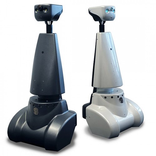
The most memorable part of the course Embedded Motion Control is the 'A-MAZE-ING PICO' challenge, in which software is designed for and implemented into autonomous robots. These autonomous robots, called PICO and TACO, should then be to able to solve a maze with the software in a real-life environment. A maze can contain loops, dead ends, open spaces and doors that automatically open and close.
PICO will be provided with a basic software layer to carry out primary functions, such as communication and movement. However, to succesfully complete the 'A-MAZE-ING PICO' challenge it is required to design a robust software architecture for the changing environment. Before the software architecture will be realized in C++ it is desired to first decide about the software practicalities. After some programming several of the software subsystems will be put to the test in an intermediate challenge. During this challenge, called the corridor competition, PICO must move through a corridor and take the first exit. With the results of the corridor competition and all its software subsystems PICO should be able to finish the maze challenge. The course Embedded Motion Control is concluded with conclusions and recommendations along with several links to parts of the actual code.
Software Architecture
The ever-changing environment requires the design of a robust software architecture. It is prefered to design this software architecture before actually programming, because it gives a clear understanding/agreement of the different functions from the start. The first step in creating the software architecture is to mention the requirements that have to be met in order to complete the corridor competition and the maze challenge. PICO should be able to finish these challenges succesfully by using components. Secondly, a list of specifications will be given to accuratly describe the robot, corridor and maze. With these requirements, components and specifications it is possible to define functions for the software architecture. The software architecture is completed by specifying the interfaces between task, skill, motion, world model and user interface. It is noteworthy to mention that the final software design in this section, which was also presented during our final presentation, is based on our initial design plan report and first presentation.
Requirements
To complete the corridor competition and maze challenge PICO has to meet the following requirements:
- Operate fully autonomous
- Avoid collisions with walls
- Robust against sensor disturbances and layout imperfections
- Update, compile, start and end software with single commands
- Corridor competition
- Move through a corridor that complies with the specifications
- Exit the corridor within the set time limit
- Recognize junctions
- Maze challenge
- Move through a maze that complies with the specifications
- Escape the maze within the set time limit
- Recognize junctions, loops, dead ends and doors
- Ring the bell at dead ends and doors
- Stand idle for a certain period of time
Components
The following components of PICO will be used to fulfill the requirements:
- Sensors
- Laser range finder (LRF) determines the distance to an object with a laser beam
- Wheel encoders (odometry) determine the position of PICO relative to a starting position
- Actuators
- Holonomic base with three omni-wheels to drive and turn
- Bell to request a door to open
- Computer
- Intel I7 processor
- Ubuntu 14.04 as operating system
Specifications
PICO, the corridor competition and the maze challenge are characterized by the following specifications:
- PICO
- Maximum translational speed of 0.5 m/s
- Maximum rotational speed of 1.2 rad/s
- LRF
- Range of 0.1 to 30 m
- Horizontal field of view of 270°
- Corridor competition
- Corners are approximately 90°
- Distance between walls can range from 0.5 to 1.5 meter
- Maze challenge
- Corners are approximately 90°
- Distance between walls can range from 0.5 to 1.5 meter
- Can contain loops, open spaces and more than one dead end
- A door area is located in front of a door and is 1.3 meter long
- Door opens when PICO is inside the door area, stands still and sends a request
More details can be found in the extended specifications.
Interfaces
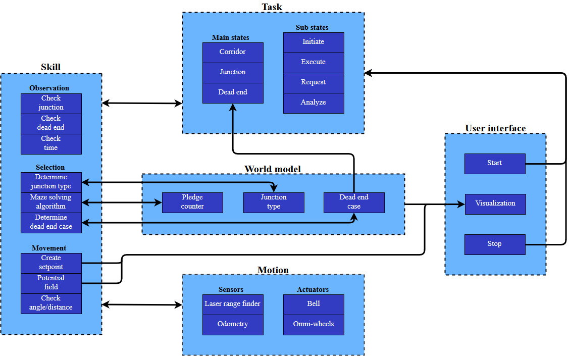
In order to complete the software architecture, a task-skill-motion framework is constructed. This framework describes primarily the connection between low-, mid- and high-level elements in the software. Furthermore, it connects the software elements to a world model and user-interface. Task contains the high-level software elements that are responsible for the strategy and high-level decision making. Skill contains the mid-level software elements that are required to realize the task. The motion part contains the low-level software elements that access the abilities of the robot. Hence, task-skill-motion correspond to the states, functions and components (actuators and sensors) of the function flow chart, respectively.
Functions
The requirements can be met with the given components and specifications by defining various functions for the software architecture. These functions typically use sensor information to determine the next actuator action, or compute a variable that is used by another function. When defining functions it is important that each function has a single and clear purpose. All the functions that are required to complete the maze challenge are visualized in a function flow chart. The colors in the function flow chart indicate how much functionality of a function is necessary to finish the corridor competition instead. This design saves time because every function used in the corridor competition is reusable for the maze challenge. The function flow chart starts every iteration with getting sensor data, and based on the state of the state machines a different part of the code is executed. A dashed line is used to illustrate which function can alter the state in a state machine. Furthermore, the main and sub state machines are initialized at the corridor, initiate and request state.
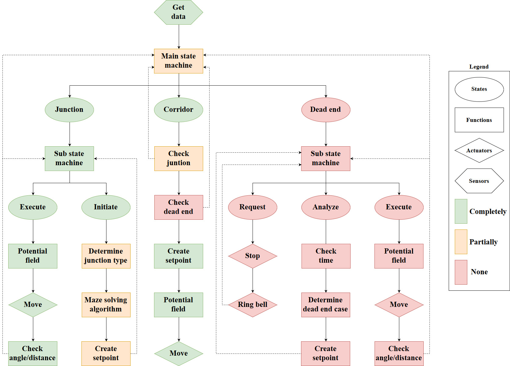
The role of each function will be clarified with three small scenarios. In the first scenario PICO is located at one end of a corridor and needs to move to the other end. PICO will do so by first getting sensor data from the LRF and odometry, and then entering the corridor state via the main state machine. The LRF data is then used to check whether there is a junction or dead end near PICO. This is not the case, so a setpoint is created in front of PICO. The setpoint and the location of the walls are then used to create a potential field. With this potential field PICO is able to move a small distance through the corridor while avoiding the walls.
In the second scenario PICO is located near a junction, but the junction has not yet been detected. Similar to the first scenario PICO will obtain sensor information, enter the corridor state and use the LRF data to determine if there is a junction or dead end near PICO. However, this time a junction is detected and the state of the main state machine is switched to the junction state. This switch ensures that PICO carries out the functions in the initiate sub state at the next iteration. Within the initiate sub state the type of junction is determined, a decision is made by the maze solving algorithm and a setpoint is created in the direction PICO needs to move. After the initiate sub state is carried out once, the state of the sub state machine is set to the execute sub state. The functions in the execute sub state are carried out every iteration until PICO has driven/turned sufficiently according to the odometry data. In other words, the main state machine and sub state machine are reset to their initial states when PICO is close to its setpoint.
In the third scenario PICO is located in a corridor with a dead end, and the dead end has just been detected. This implies that PICO will carry out the functions in the request sub state at the next iteration. The request sub state ensures that PICO stops moving and that it rings the bell. After the request sub state is carried out once, the state of the sub state machine is set to the analyze sub state. The first function in the analyze sub state is used to wait a predefined amount of time for a possible door to open. When the time has passed the LRF data is used to determine whether it was a door or dead end. Based on its findings a setpoint is created in front or behind PICO in case of a door or dead end, respectively. After the setpoint has been created, the state of the sub stame machine is set to the execute sub state. Finally, the functions in the execute sub state are carried out every iteration until PICO has driven/turned sufficiently according to the odometry data.
Software Practicalities
In order to keep the software components clear and keep modularity easy, several design decision need to be made before creating the actual functions of the software. The main flow and structure of the code has been designed and explained above, but this needs to be translated into c++.
First of, the way the code flows through the several possible states needs to be determined. This is done using a so-called state machine. By simply changing the state of the code when certain conditions are met, the code will run a different part during the next iteration. As can be seen in the flow chart above, 1 main state machine is used for the corridor, junction, and dead end states. Moreover, the junction and dead end state have an internal state machine of respectively two and three states to determine in which phase of the procedure the code is. By using a state machine, only a couple of if statements are needed to switch between the states. This keeps the code clear and faster.
Secondly, choices need to be made regarding the way data is stored. To keep functions modular, all data need to be saved in a similar way to prevent miscommunication between functions. To do this, a main header file has been created in which certain classes are defined. This file is then imported within all the other functions to guarantee the same definitions in each function. In particular, the following custom classes have been created:
- Point: the point class contains two doubles indicating its x- and y-coordinate. The x-direction is defined as the direction when PICO looks straight ahead. The y-direction is perpendicular to this.
- Vector2: a vector class is already available in c++, but a second one is created that is defined by 2 points. These points indicate the start and end point of the vector.
- OdomData: to prevent odometry data to be called twice within the same iteration (which would have major consequences), a class has been created that stores all the odometry data of that iteration which is called only once each iteration. The OdomData class thus contain three doubles indicating the difference in x-, y-, and theta-data compared to the previous iteration.
- Forces: the forces class is used by the potential field and visualization. Since a function can only return a single value or class, this class has been created in order to return three different forces. These forces are the attractive, repulsive and total force. Each of these forces is a vector which can then be used to drive PICO.
The final choices that need to be made are about the way PICO's sensor data is handled and the way PICO is driven. The laser data PICO imports is limited to a set distance in each function. When the data is further than this distance, the data is ignored since it is too far away from PICO. This has been implemented since several functions registered junctions, doors and setpoints way too early thus causing PICO to go into the corresponding state prematurely. Another issue involved PICO registering multiple junctions at once, thus messing up the junction type detection. Several tests have been done to determine the correct distance at which the data should be limited, and in the maze challenge 1.3m has been used. Regarding the driving of PICO, the decision has been made that the maximum translational speed is limited to 0.3 m/s. This way PICO has more time to gather data and make decisions. The negative part of this decision is obviously the fact that the time to find the exit would be larger. The code did however become more robust because of the lower speed.
Software Subsystems
In this section, all the important functions are explained that are used in the main part of the code. First of the way PICO recognizes junctions is explained, and the possible types of junctions are shown. After this, the way PICO sees and handles doors is elaborated and visualized. The section then continues with the setpoint detection and the turning of PICO. After this the potential field and pledge algorithm are explained, and finally the visualization is treated.
Junctions
The junction handling is done in two checks. The first check is executed in the corridor state in which a detection takes place. This detection tells whether there is actually a junction of not. this is the check junction. If there is a junction at all, the second check within junction state checks the type of junction. On the basis of these checks, a decision will be made and a setpoint will be determined. Within this part, the check junction and the detect type junction will be described.
Check Junction
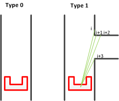
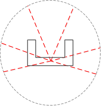
The first check for junction handling is the check junction script in the corridor state. This detection return whether there is a junction or not. It does, however, not detect the type of junction. This has been done consciously due to the switch between the corridor state to the junction state. If there is a potential junction, the state switches from corridor to junction where the detection of the type takes place. To detect a junction, the laser range finder (LRF) data is being used. A minimum distance between the beams is being set to 5 cm. For robustness, the beams lengths of three following beams are compared with each other. If the length of the first indicated beam minus the length of the next beam is greater than the set value of 5 cm, and the initial beam i minus the second and third beam are greater than this 5 cm, PICO will detect a junction and will return 1. This has been done for a bundle of beams on the right side, left side and in front of PICO. The detection has been visualized in the next figure. PICO's laser range can also be found on the next figure. If a junction is detected, PICO also needs to know what type of junction this is. This will be described in the next section.
Detect type junction
Within detect type junction, PICO detects the type of junction it encounters. First, the types of junctions has been characterized. These are as follows:
- 0 Type undetected
- 1 Corridor with a sideroad to the right
- 2 Corridor with a sideroad to the left
- 3 T junction
- 4 Full junction (Crossroad)
- 5 Dead end
- 6 Turn right
- 7 Turn left
The junctions can be found in figure below:
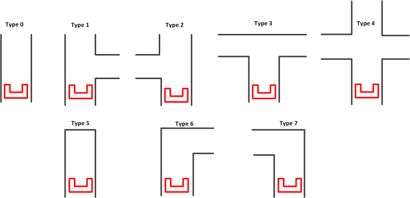
Again, to detect the type of junction, PICO uses its LRF-data on the right, left and front of PICO respectively. To reduce the radius of the LRF-data, a global variable VIEW_DIST has been introduced. This variable is set to 1 meters. This means that the PICO can only see for a distance of 1 meters. First, the values for right, left and straight are initialized as 0,0 and 1 respectively. Within this 1 meters, PICO constantly checks the difference in lengths of the first beam with the second and third beam for robustness. If this value exceeds the defined value of 5 cm, the right and left variable are set to 1 and a new maximum view distance is calculated with respect to the angle between the beams, the length of the beams and the distance to the wall which is set to 1.3 meters. This new view distance is than used in the detection of the front side of PICO.
For the front detection, PICO checks whether the beam length of the LRF-data is lower than the new view distance and larger than the defined variable MIN_DIST which is 1 cm. This last part is added due to the fact that the LRF-data becomes very small when PICO detects outside the parcour. If the conditions are met, the straight value is set to 0. These perceptions are than translated to junction types and these are stored in an array. The method can be found in the script.[1]
For robustness, an iteration counter has been set in the mains script. This counter is used in the junction type detection. If the iteration is larger than six, thus the type junction stored in the array is checked six time, than the type of array is checked for the first six iterations. If for all these iterations the output of the junction type remains the same, than the output of the detection is this particular junction type. During the experiments, it has been noticed that for instance the first 4 iterations the junction types fluctuated and a less accurate detection was observed. To tackle this problem, this method has been implemented in the script.
A failsafe is added for when PICO incorrectly detects a dead end because he does not observe any vertices (for instance in an open space). If this is the case, than the type junction is set to 6 and 7 respectively which means that PICO should turn to the left or right according to the situation.
 |
Potential Doors
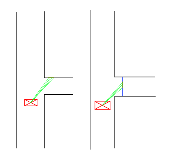
The detection and handling of potential doors is important to be able to find and pass the door that might be in the maze. Potential doors are detected by the main script as a specific type of junction.
Door Recognition
There are two possible types of doors PICO can recognize in the maze. The door is namely either located at a dead end, or placed to the side of the corridor. The second possibility is visible in the figure on the right. The way PICO recognizes a dead end is fairly simple. It checks all its laser data, and if all distances are lower than a certain minimum (0.5m) PICO decides that there are no possible gaps to move to, and it is thus a dead end. This initializes the door procedure.
The way PICO recognizes side doors is visualized in the figure on the right. After PICO has seen a junction, and thus a gap on either side, PICO will check if the gap is actually a corridor or a door. This is done by comparing the laser data as shown in the figure, as checking if the difference in the data is mostly in the x-direction or the y-direction. As can also be seen in the figure, a green line in the x-direction indicates a door, while a line in y-direction means the gap is a corridor. If PICO determines that the gap is a potential door, the door procedure explained above is executed.
Door Procedure
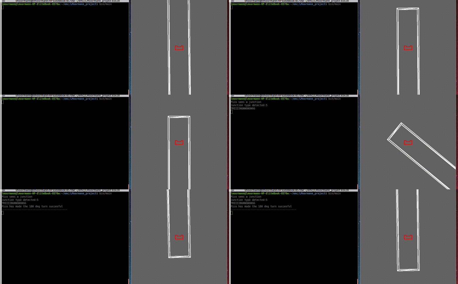
When a dead end is detected, the case is switched to potential_door. There is a check variable, which prevents the reaching of this state if a door has been detected and passed in the past. case consists of three different sub-cases which make sure of the following:
- Drive up to the door
- Turn PICO so its forward direction is perpendicular to middle of the potential door.
- Initiate the potential door procedure
The door procedure calls a function which rings the bell, waits for five seconds, and subsequently checks whether there was a dead end whose wall still stands, or whether there was a door that has been removed. The function returns either door or dead end back to the main script, which continues with this information. If the potential door turns out to be a dead end, a 180°-turn is initiated by switching to the appropriate state and reinitializing the setpoints and odomotry, after which normal operation is resumed. If there was a door, PICO will enter through it and continue normal operation. Furthermore it is recorded that a door has been passed, so that this procedure will not be performed again.
 |
 |
Setpoints

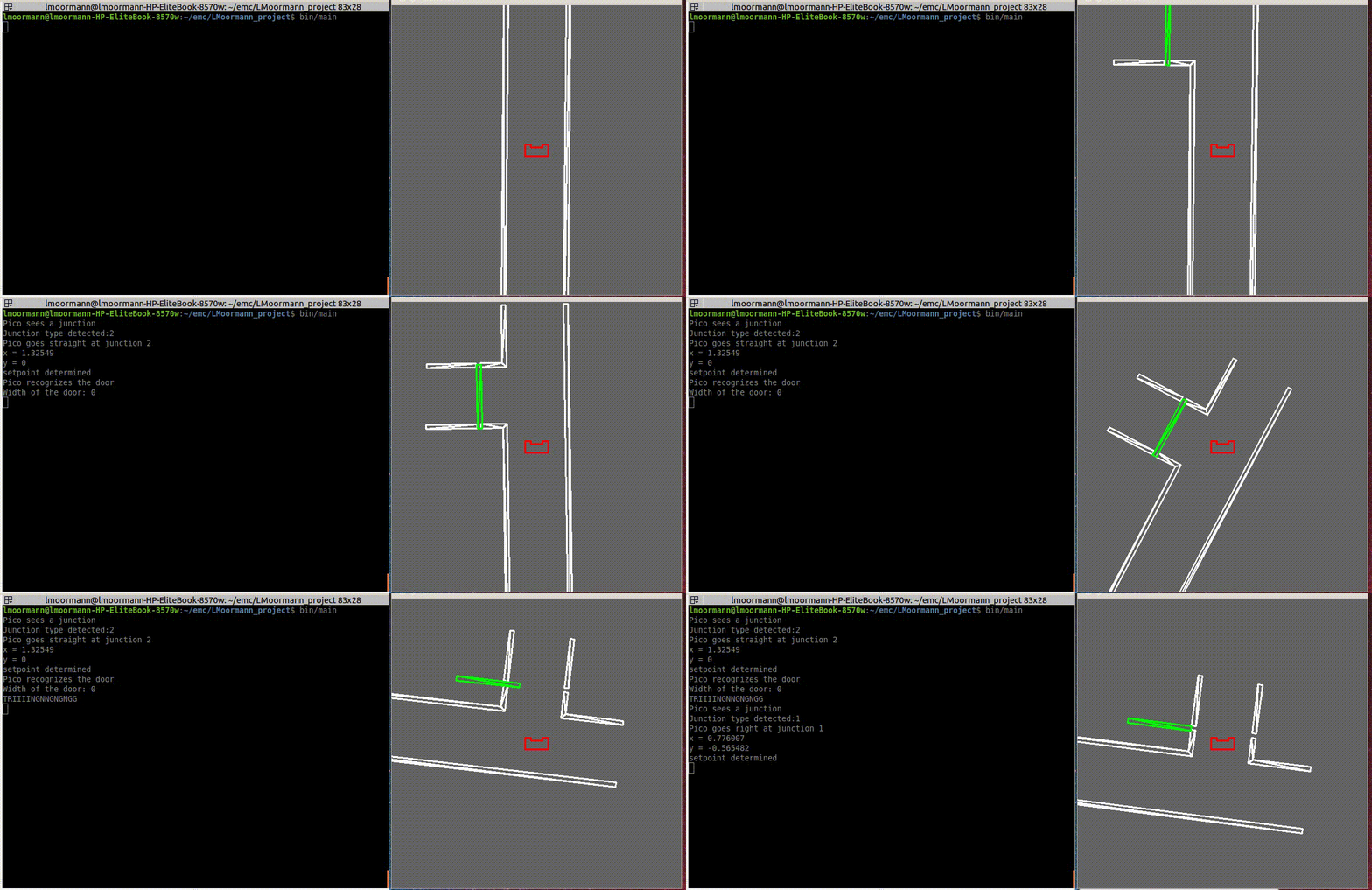
The setpoint detection function is used after the junction type is recognized and PICO has made a decision on which way to go. The function first finds the required corner points corresponding to the junction type and then converts the data into the correct setpoint data. The first figure on the right shows an example of a junction type and the required points to determine toghether with some laser beams.
The green points in the figure represent the points PICO will recognize. The blue points are the setpoints PICO will use to take the corner. The locations of the these blue points are calculated from the data of the green points.
The left green point is the first point PICO will look for. To find this, it will go through a part of its laser data and compare the distances of subsequent data entries. In this for-loop, the distance of the current laser data (called i) and the distances of the three following data points (i+1, i+2, i+3) are compared. When the difference is higher than a set minimum (5 cm), PICO will recognize this as a gap in the sidewall and save the corresponding angle and distance. The left green point corresponds to the data point i, and the right green point is data point i+3.
Once the data of the green points is found, this data is converted into an offset in x and y direction. This offset is measured with PICO as origin, where the x-direction is the direction PICO is driving in, and the y-direction is perpendicular to this. The offsets are calculated by first determining the angle at which the data point lies, after which trigonometry is used to find the offsets. The equations below show the formulas used in the code.
- [math]\displaystyle{ \theta }[/math] = ([math]\displaystyle{ \theta }[/math]min + [math]\displaystyle{ \theta }[/math]increment * [math]\displaystyle{ i }[/math]) * 67.5 * [math]\displaystyle{ \pi }[/math] / 180
[math]\displaystyle{ \theta }[/math]min is the smallest angle PICO can see, [math]\displaystyle{ \theta }[/math]increment is the difference in angle between two data points, [math]\displaystyle{ i }[/math] is the data entry corresponding to the left green point. Since the angle data of PICO ranges from -2 to 2, which corresponds to -135 degrees to 135 degrees. This thus results in a factor 67.5 that is incorporated.
- [math]\displaystyle{ }[/math] x = ([math]\displaystyle{ r }[/math]1+[math]\displaystyle{ r }[/math]2) / 2 * cos([math]\displaystyle{ \theta }[/math])
[math]\displaystyle{ r }[/math]1 and [math]\displaystyle{ r }[/math]2 are the distances in the laser data of the left and right green points respectively.
- [math]\displaystyle{ }[/math] y = ([math]\displaystyle{ r }[/math]1+[math]\displaystyle{ r }[/math]2) / 2 * sin([math]\displaystyle{ \theta }[/math])
The lower blue point in the first figure is then determined by calculating the point exactly between the two green points. The data for this blue point is once again saved as an offset in x- and y-direction. The offsets of the upper blue point is then simply calculated by taking the same x-offset as the lower blue point, and setting the y-offset to 0.
This example is obviously only applicable when PICO needs to take a turn to the right. The same procedure can however be used when the turn is to the left, but the data range used to find the setpoints is then adjusted.

The final option for PICO is to go straight at a junction. The third figure shows where the setpoints are placed in that scenario. The calculation of the setpoints is done in the same way as before.
Turning
If PICO is in the turning state, it can have two options. The first option is to drive straight and the second one is to make a turn. If the first option is the case, PICO uses only the setpoint which was explained as last in section about setpoints. It will keep on driving straight until the specified distance of the setpoint is met and after that it returns to the main corridor state.
If the Pledge algorithm chose to make a turn at a specific junction the first setpoints from the previous section are used. The first step is to drive straight until PICO has driven the right amount of distance. After that PICO stops and turns for either +90 degrees or -90 degrees and check with the odometry data if the angle is finished. After this step PICO drives forward until either the distance of the left beam of PICO or the right beam of PICO (which depends on the turn type) is smaller than 0.75 meter. After this the state gets changed into the main corridor state.
Potential Field
PICO uses a potential field to drive through the maze. This prevents PICO from colliding with the walls and it automatically alligns PICO in a corridor. The potential field works with two virtual forces which are the attractive force and the repulsive force.
The attractive force is always equal to the relative distance to the setpoint. The repulsive force depends on the distance between the walls. Each range from the laser data is transformed into a vector and than scaled with the following equation:

After that all the single repulsive vectors are added to each other which results in the final repulsive force. The parameters of this equation have been determined while testing with PICO at the test sessions. The forces used in the potential field are shown in the Figure below:
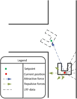
Later on some values in the potential field where tweaked because PICO was zigzagging too much in a straight corridor. Also an extra argument was added to the potential field function called “turning”. This argument was equal to 1 if PICO was in a turning state and it was equal to 0 if it was just driving straight. The reason for adding this extra argument was that in the turning state more velocity was needed in the y-direction and also more rotational speed was needed.
The final script which was used for the potential field can be found here.
Pledge Algorithm
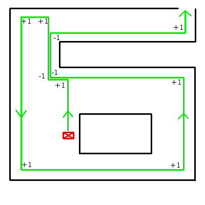
To find the exit of the maze the Pledge algorithm is chosen. The Pledge algorithm is suitable for maze problems where the starting point is within the maze and the exit is at the border of the maze. The modified wall following algorithm has a preferred direction which allows the robot to circumvent obstacles and directs the robot towards the outer walls of the maze. By tracking the number of perpendicular turns the algorithm keeps track of the direction. The Pledge algorithm is chosen because it is suited for the problem and simple to implement in the code. The algorithm can be based on either a left- or right-hand wall follower. There is no significant difference between the two versions. Which version can find the exit faster depends on the maze and the location of the entrance and exit. Since the maze is unknown, the choice to use a right-hand wall follower in the maze challenge is arbitrarily.
The rules for the right-hand Pledge algorithm are:
- When PICO is driving in the preferred direction; when the counter is 0: try to go straight (+0), then try to go left (+1), or else, turn around (+2).
- When PICO is driving in any other direction; when the counter is not 0: try to go right (-1), then try to go straight (+0), then try to go left (+1), or else, turn around (+2).
An example of the algorithm can be seen on the right. The algorithm is implemented in the 'make decision' function by applying the rules to the different junction types. For every junction type and counter setting(zero or non-zero), the decision which direction to go is predefined. In another function the counter is updated, depending on de selected direction.
Visualization
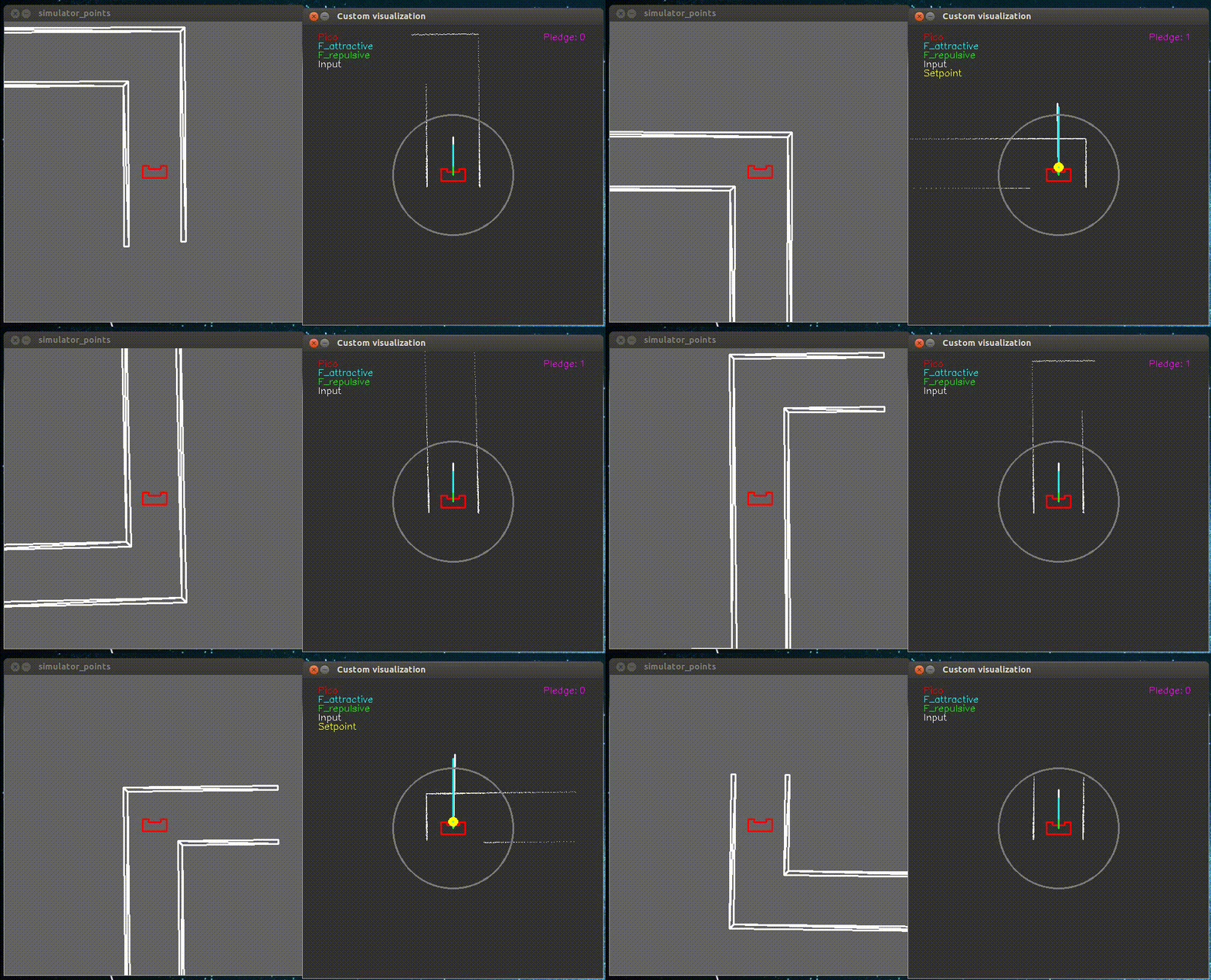
A custom visualization has been made to show the forces of the potential field, the maximum viewing range of PICO and the location of the setpoint. The function “show_canvas” must be called to update the visualization. This function has multiple inputs which are: the laser-data of PICO, the forces class and the location of the setpoint.
In the video below on the right the custom visualization is shown with in the top left corner a small legend and on the top right the pledge counter. The white dots represent the laser data and the gray circle around PICO is the maximum viewing range.
The three forces which are shown are: the attractive force (in blue), the repulsive force (in green) and the total force, which is the sum of the attractive forces and the repulsive forces (in white). These forces are returned by the potential field in a class called “forces”. The reason for this is that a function can only return one value or class in our case.
A code snippet of the code used for the visualization can be found here.
 |
Corridor Competition
The purpose of the corridor competition is to test part of the software architecture halfway through the course. During this intermediate challenge on the 24th of May PICO had to move through a corridor and take the first exit. The location of the exit and dimensions of the corridor were not given in advance, but were determined by the organisation at the time. For the first attempt we used a version of the software that was actually tested on PICO the day before. During this test it became clear that this version had sometimes difficulties making a turn at the T-junction. Nonetheless, we decided to use this version of the software and hoped for the best. The performance of PICO during its first attempt in the corridor competition is shown in the following video.

In this video it is visible that PICO is able to correctly move through the corridor, but that it pauses before taking the wrong exit. PICO was standing still at the T-junction because it was unable to create a setpoint in the initiate sub state. This issue arises when only the first corner point of the T-junction is detected. A way to solve this problem is by permanently increasing the range at which the LRF data is neglected. However, this solution is undesirable because PICO can then detect multiple junctions at the same time while moving through the corridor. A better solution would be to momentarily increase the range at which the LRF data is neglected when the first corner point is detected, so the second corner point can be found.
For the second attempt we used a version of the software that was only tested in the simulation environment due to lack of time. A key difference between the two versions is the method how a setpoint is created in the initiate sub state. In this version the setpoint is created with the aforementioned solution of momentarily increasing the range at which the LRF data is neglected. The performance of PICO during its second attempt in the corridor competition is shown in the following video.
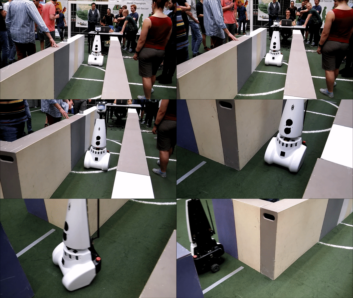
In this video it is visible that PICO is able to correctly move through the corridor, but that it slightly touches the wall before taking the correct exit. PICO makes contact with the corner of the wall because the setpoint was placed too far to the right. In addition, the potential field was not yet tuned for the junction state. These two shortcomings in the software were eventually corrected during a test session in the week after the corridor competition. PICO managed to complete the corridor competition with a second attempt in approximately 13 seconds, but a 5 second penalty was given for slightly touching the wall. If PICO was able to avoid a collision with the wall, we would have been first instead of second.
Maze Challenge
At the end of the course the entire software architecture, as described in the software design, is tested in the maze challenge. During this final challenge on the 14th of June PICO had to move through a maze and find the exit. The location of the exit and layout of the maze were not given in advance, but were determined by the organisation at the time. For both attempts we used a version of the software that was actually tested on PICO the days before. During these tests it became clear that most of the functions in the software were working properly. However, a slight error in the other functions could have a major impact on the overall performance. It was unfortunately not possible to fix or redesign these unreliable functions for the maze challenge due to time limitations. The performance of PICO during its first attempt in the maze challenge is shown in the following videos.

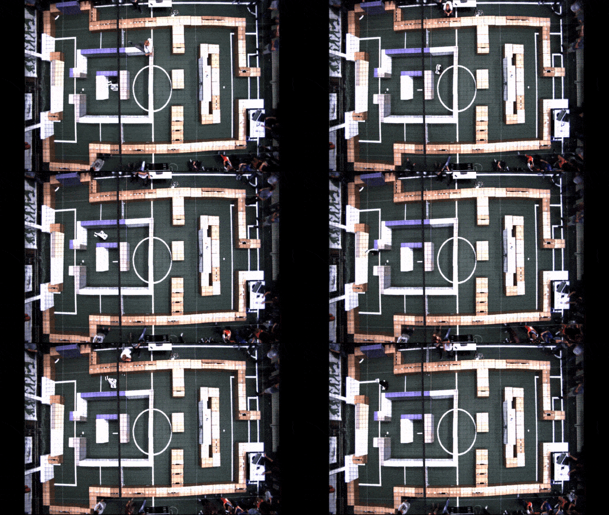
In these videos it is visible that PICO is able to move through the maze while avoiding the walls, but that it makes a U-turn when it just opened and passed through the door. PICO made this decision because the counter used by the Pledge algorithm was off. This issue arises when PICO makes unnecessary turns in a corridor area of the maze. A way to prevent these unwanted turns is by ensuring that PICO moves straight through a corridor area. This requires that the setpoint after a corner is placed at a more suitable location by means of an iterative testing process.
The first attempt was stopped by the group when PICO was moving back to its starting position. PICO would be able to eventually reach the exit, but it would take a considerable amount of time. For the second attempt we used the same software as the first attempt because we anticipated that PICO would be able to make the corners more accurately this time. The performance of PICO during its second attempt in the maze challenge is shown in the following videos.

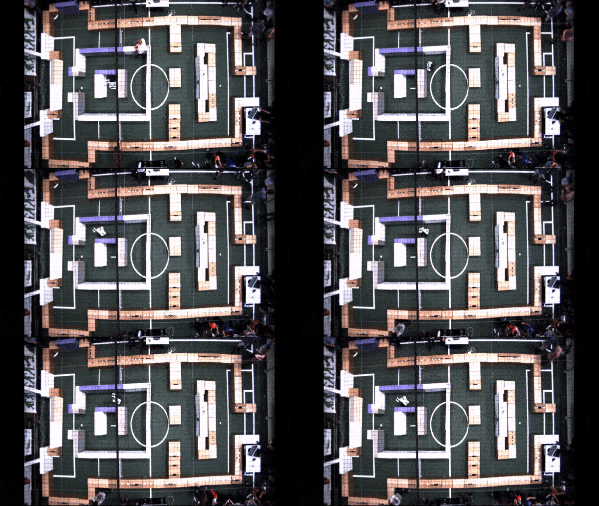
In these videos it is visible that PICO is able to move through the maze without collisions, but that it is unable to navigate out of the inner loop area. PICO got stuck in this area because the misalignment with the walls was too great for PICO to correct. This problem was again caused by the misplacement of the setpoint after a corner. We were unfortunately unable to complete the maze challenge due to this shortcoming in the software. If the project was to be continued past the deadline, our priority would be to improve the create setpoint function.
After the maze challenge, the same maze was tested in the simulation. This way it could be proven that the code is indeed able to solve the maze, albeit only in the simulation. The video below shows how PICO is eventually able to solve the maze. Once again, some errors were introduced by the setpoint detection, but based on potential fields PICO was able to straighten itself and find the exit. It should be mentioned that the only part of the code that was changed between the maze challenge and the simulation is the viewing distance of PICO. This was changed from 1.3m to 1.0m to increase robustness in the simulation. PICO was able to solve the maze in the simulation in 4 minutes and 19 seconds.
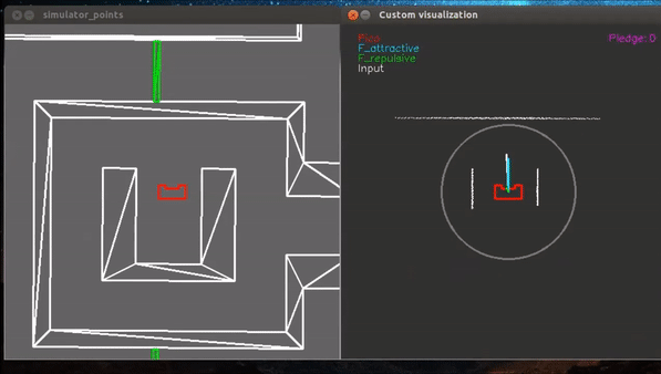
Conclusions and Recommendations
The goal of this project was to create an organized code that would make PICO solve any maze following the specifications. It is clear that the solving of the maze was not succeeded during the maze challenge. The same code and maze were however later tested in the simulator, which showed that PICO is in fact able to solve the maze using the original code. The problem was the robustness of this code. Some conclusions can however be drawn about which parts of the code worked correctly, and recommendations can be made for the parts that could be improved.
First, the potential field worked as expected. In the corridor challenge some problems were noticed regarding the potential field, namely hitting the wall. After this challenge the potential field was tweaked some more, after which PICO never hit a wall again. This is also noticed in the maze challenge. Even though PICO’s decisions were not always correct, it never hit the wall.
Secondly, the junction type detection worked well. During the programming and testing phase of the project, many problems were encountered for the detect_type_junction function. PICO would recognize the wrong types of junctions to often to reliably solve the maze. Elaborate testing and tweaking however resulted in a more robust and reliable function that was also used in the maze-challenge.
Finally, the door recognition and procedure worked perfectly. As is also visible in the maze-challenge, PICO recognized the door flawlessly after which the door procedure was executed. PICO rang is bell and correctly noticed that the door opened, after which it drove through. The side-door detection could not be tested during the maze-challenge, but during the individual tests it worked every time.
The main problem in PICO’s code and also the reason the maze challenge was not finished successfully is the setpoint detection. As can be seen in the maze challenge, PICO sometimes takes its corners too sharply and potential fields kick in to avoid wall collisions. In order to make the code more robust, a more elaborate setpoint detection should be implemented. Possible ways to do this is by looking at all the laser data PICO sees and creating walls and corners from this data. This way the detection is more robust since it is dependent on all the data instead of small ranges of data. It also eliminates the use of the data filter with a range of 1.3m. The choice to use this range was necessary for the way setpoints and junctions are recognized, but is not ideal.
A second part that could be improved in the code is the handling of open spaces. Right now PICO has no special functions and states to detect and pass these open spaces. More elaborate research and testing should be done to decide on a way to handle these open spaces.
Regarding the structure of the code, most decisions resulted to be positive. The use of a task-skill-motion diagram and a corresponding flowchart helped tremendously in creating a clear code that could easily be extended. All functions named in the flowchart are created in a separate function file to enable working on multiple parts of the code at the same time. The design of the flowchart also enabled us to expand on the code of the corridor challenge instead of having to restart.
One of the aspects that could have done better in the code structure is the use of magic numbers. Magic numbers are globally defined values that can be requested in each part of the code. A lot of magic numbers were used, but looking back at the code showed that too often actual numbers were used instead of globally defined ones. This does not at all break the code, but it would be a lot clearer and more accessible if magic numbers were used in these cases as well.