Mobile Robot Control 2024 Optimus Prime: Difference between revisions
No edit summary |
|||
| Line 84: | Line 84: | ||
=== A* algorithm === | === A* algorithm === | ||
=== Probabilistic Road Map (PRM) === | |||
[[File:Inflated walls with dilation size equal to 1.png|thumb|Inflated walls with dilation size equal to 1]] | |||
=== <u>Probabilistic Road Map (PRM)</u> === | |||
* Wall inflation | |||
[[File:Inflated walls with dilation size equal to 2.png|thumb|Inflated walls with dilation size equal to 2]] | |||
To inflate the walls dilation is being used. To do that, the map colors are first inverted since Opencv inflates white parts of the binary image from that the dilation size variable can be used to adjust the size of how much the wall is inflated. The maps with inflated walls can be seen to the side. | |||
After that map is inflated it is transformed back to its initial color scheme. | |||
* Distance from other points | |||
To check if there is no other point around each newly created point a square are of 0.1x0.1 m is being checked and if there is already a point in that area the new node is being discarded. | |||
* Check for valid edge | |||
To see if the vertex is valid to checks are being performed. First the distance between the nodes is being checked by computing the absolute value of a difference of the x and y variables of 2 nodes and then taking a square root of a sum of those values squared. | |||
The other check that is being performed is seeing if there is a wall between the two nodes. To do that a line between two points is being created using Bresenham's algorithm, it creates all the points and is used to check if there is a black point along the path. If the line encounters the black point it is marked as invalid and the edge between the two points is not created. | |||
== '''Exercise 4 - Localization''' == | == '''Exercise 4 - Localization''' == | ||
Revision as of 17:07, 21 May 2024
Introduction
We are Optimus Prime, a team of six members applying various control techniques and coding skills to optimize a robot for restaurant environments. Our goal is to enable the robot to efficiently deliver orders from the kitchen to the tables, even when faced with various obstacles. This project focuses on ensuring precise and reliable performance, ultimately improving service efficiency and the overall dining experience.
Group Members
| Name | student ID |
|---|---|
| Yuvan Dwaraga | 1563793 |
| Wiktor Bocian | 1628798 |
| Ramakrishnan Rajasekar | 1979027 |
| Ariyanayag Ramesh Skandan | 2012618 |
| Abhir Adiverekar | 1984136 |
| Suryakumar Hariharan | 1974076 |
Exercise 1 - The art of not crashing
This exercise aims to enhance our understanding of control techniques and obstacle avoidance algorithms.
Solution 1
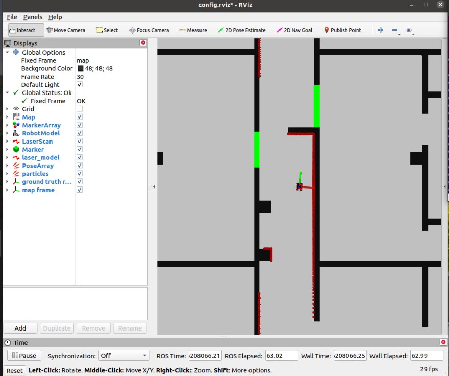
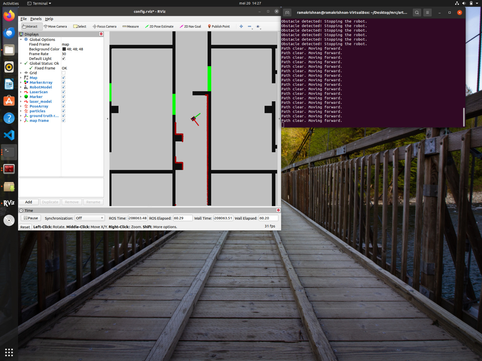
The odometry and laser data were obtained based on the instructions from the manual, enabling the robot to be aware of its surroundings. Although this sensor data does not provide instructions for the robot to stop or go when an obstacle is on its way, a discussion was held to include a constant safe distance value, which ensures that the robot maintains a safe distance from obstacles and avoids collisions. Loops were also introduced as the robot operates to check whether the obstacles are close to the robot or not. Specifically, if an obstacle is detected within a certain range less than the predefined safe distance (0.5 meters) the robot will come to a halt. This algorithm ensures that the robot can navigate in its surroundings safely.
Solution 2
Advancements to the previous solution were made by introducing rotation values and forward motion value to enhance the robot's performance. These values were effective when the obstacle is too close to the robot. The stoppage of the robot comes into play and the rotation values allow it to rotate with movement restriction and later it allows the robot to move in the forward direction with constant units. This approach ensures that the robot not only stops to avoid immediate collisions but also actively seeks a safe route forward. Overall, the combination of a constant safe distance, rotation and forward actions allows the robot to perform more efficiently.
Learnings from solution
The robot's performance in this case was evidenced in both simulation and in practical sessions. Alterations in the code were made so that, in case of the obstacle detection, the robot was made to move in the x direction in adherence to the safe distance.
Practical session
I am not able to link with videos .mp4 files maybe only jpeg are allowed. Not sure though.
Artificial potential fields
Motivation
Our motivation for choosing the artificial potential field algorithm lies in its effectiveness for real-time obstacle avoidance and smooth navigation. This approach enables our robot to dynamically manoeuvre around obstacles by leveraging attractive and repulsive forces, ensuring efficient path planning.
Solutions
Learnings from each solution
Visual representation of sim
Practical video
Pros and cons
Dynamic window approach
Motivation
Our motivation for choosing the Dynamic Window Approach (DWA) method is its ability to optimize both velocity and trajectory in real-time for safe and efficient navigation. This algorithm allows our robot to dynamically adjust its path by considering its kinematic constraints and the surrounding obstacles, ensuring precise and responsive movement.
Solutions
Learnings from each solution
Visual representation of sim
Practical video
Pros and cons
Exercise 3 - Global path planning
A* algorithm
Probabilistic Road Map (PRM)
- Wall inflation
To inflate the walls dilation is being used. To do that, the map colors are first inverted since Opencv inflates white parts of the binary image from that the dilation size variable can be used to adjust the size of how much the wall is inflated. The maps with inflated walls can be seen to the side.
After that map is inflated it is transformed back to its initial color scheme.
- Distance from other points
To check if there is no other point around each newly created point a square are of 0.1x0.1 m is being checked and if there is already a point in that area the new node is being discarded.
- Check for valid edge
To see if the vertex is valid to checks are being performed. First the distance between the nodes is being checked by computing the absolute value of a difference of the x and y variables of 2 nodes and then taking a square root of a sum of those values squared.
The other check that is being performed is seeing if there is a wall between the two nodes. To do that a line between two points is being created using Bresenham's algorithm, it creates all the points and is used to check if there is a black point along the path. If the line encounters the black point it is marked as invalid and the edge between the two points is not created.


