Embedded Motion Control 2018 Group 7
Group Members
| TU/e Number | Name | |
|---|---|---|
| 0833049 | Sam Roovers | s dot roovers at student dot tue dot nl |
| 0886654 | Siebrand Keja | s dot c dot keja at student dot tue dot nl |
| 1022624 | Milan Haverlag | m dot a dot haverlag at student dot tue dot nl |
| 1279637 | Piyush George Alexander | p dot g dot alexander at student dot tue dot nl
|
Initial Design
The Initial Design document can be found here : File:Emc-designrequirements.pdf
Escape room competition
To escape the room, PICO will first scan its surroundings. By the use of a corner detection program the exit is determined from two laser sets (from the front and back). PICO aligns with the angle at which the exit is detected and will drive forward. A potential field must make sure that PICO does not hit any walls.
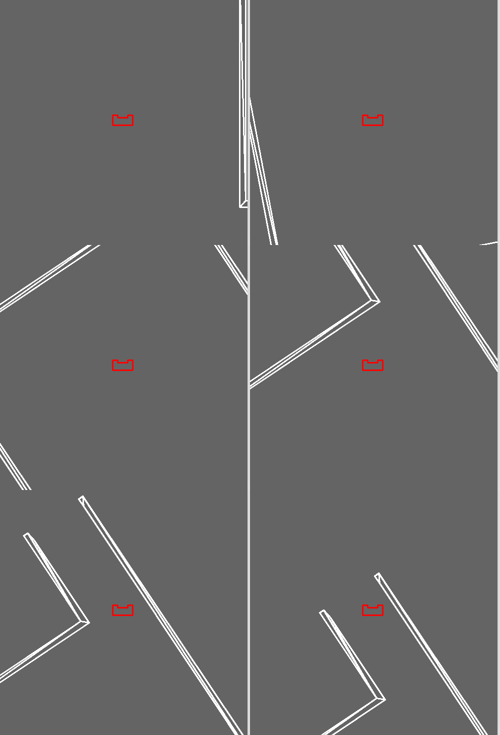
Simulation for the Escape room challenge is shown below.
Exit detection
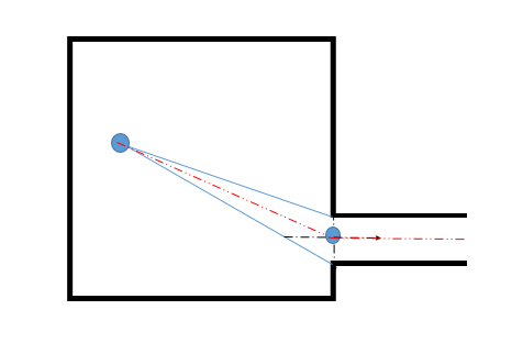
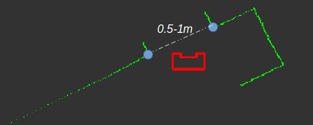
For detecting the exit, the range from the laser data was considered. PICO does a 360 degree scan and detects an exit point based on distance criteria, i.e. if the distance between consecutive sections is within the exit door tolerance ( 0.5-1 m). After detecting the two points, it searches for the point right in the middle of the detected points, which would be a waypoint for PICO to drive to, followed by which it would drive till the exit is reached.
Potential field method
In order to prevent PICO from crashing into the walls, obstacle avoidance is needed. For this it is chosen to implement potential field method. The potential field method works by combining a attractive force towards a desired set-point with repulsive forces generated from obstacles.
The Attractive force is calculated from the distance between the robot and the set-point. [math]\displaystyle{ r_{att} = \sqrt{(x_{set}-x_{PICO})^2+(y_{set}-y_{PICO})^2} }[/math] and the angle: [math]\displaystyle{ \alpha_{att} = tan(\frac{x_{set}-x_{PICO}}{y_{set}-y_{PICO}}) }[/math]
The attractive force is calculated using a proportional controller:
[math]\displaystyle{ F_{att} = r_{att}*K_{att} }[/math]
The repulsive forces are calculated by taking the inverse of the distance to the wall measured with the laser range finder with the following formula: [math]\displaystyle{ r_{rep}(i) = \sqrt{(x_{wall}(i)-x_{PICO})^2+(y_{wall}(i)-y_{PICO})^2} }[/math] [math]\displaystyle{ F_{rep}(i) = \frac{K_{rep}}{r_{rep}(i)^3} }[/math]
The attractive and repulsive forces are then split in their x and y parts. Their respective x an y parts are then added together:
[math]\displaystyle{ F_{tot}(x) = F_{att}(x) + \sum{F_{rep}(i)(x)} }[/math] [math]\displaystyle{ F_{tot}(y) = F_{att}(y) + \sum{F_{rep}(i)(y)} }[/math]
These Forces are then used to determine where PICO should drive to.
Problems with the potential field.
During testing the potential field proved unreliable. When close to a wall, Pico could get in a deadlock or start behaving erraticaly. If a way-point was set inaccurately, The potential field would cause PICO to get stuck next to a wall. It was decided to not implement the potential field on the hospital challenge but instead focus on gaining more accurate way-points. with properly set way-points coupled with a localization algoritmh, Pico would stay away from walls by itself and a potential field wasn't neccesary anymore.
Shortcommings
Due to time constraints the following features are not implemented which would have made the escape room routine a lot better.
- the positioning of a waypoint in front of the exit with enough clearing from the walls to drive to.
- alignment with the corridor after the waypoint has been reached.
At the Escape Room Competition
At the Escape room competition we face a segmentation fault, which was mainly due to reading the laser data seperately in different functions into arrays. Now only one copy of the laser data is maintained in the world model for the final architecture. This is being read by the other functions and updated.
Major take-aways
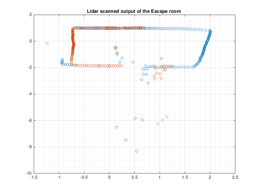
The scan made by PICO for 360 degrees in the Escape room during the test session was identified and later used as a reference for the hospital challenge. The data points in the real world were used as a reference in order to filter the laser data.
From the scanned data we decided to take one data point for every degree and maintain scan only upto 180 degrees.
The major problem that was resolved was multiple reading of laser and odometry data. This was only done once, and later updated and only a single copy was maintained in the World model for all the functions in the program to use.
Hospital challenge
Final Software Architecture
Interface
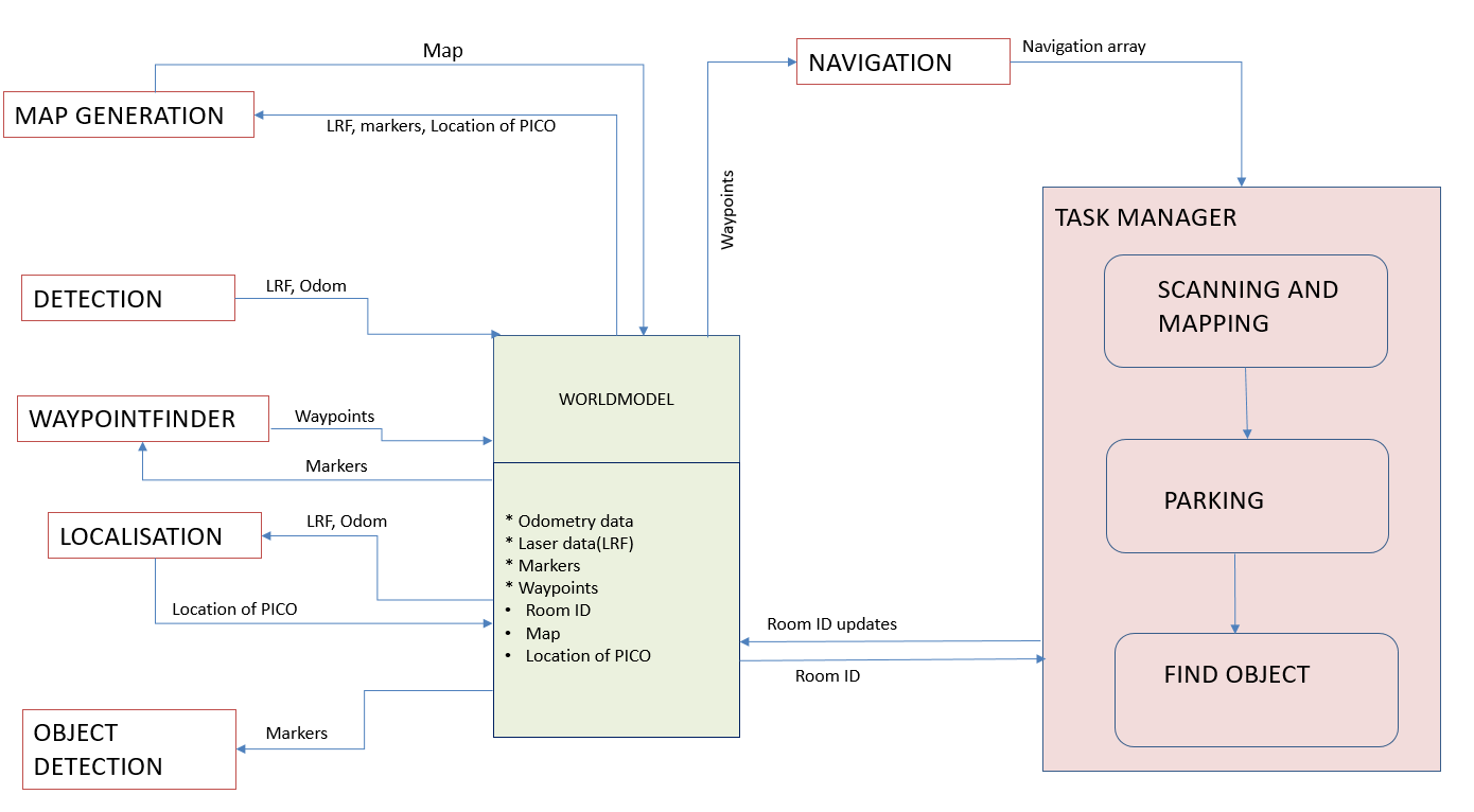
The figure below shows the data flow of our code. The core of the code is the world model.
Information processed is stored here, and action taken are based on information of the world model.
The world model is depicted by the green box in the centre. To the right the states inside the code can be observed.
Each state uses data from the world to make decisions about the next action to take. Those actions are defined as functions,
and those can be seen on the left. These functions are called in several states inside the taks manager code.
The arrows connecting the several blocks indicate the data flow, receiving and sending. The data exchanged indicated
above the arrows.
Scanning and map
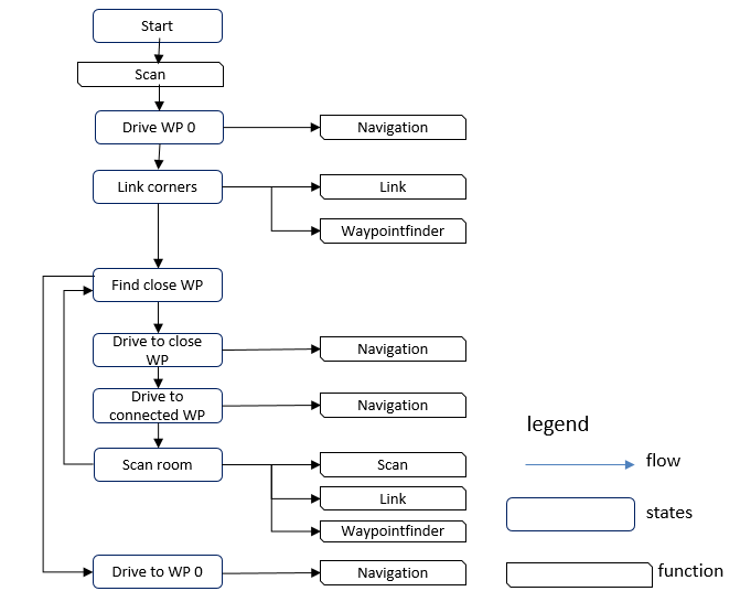
The first part of the challenge consists of mapping the hospital. The program to do this consists of the following steps. The steps are schematically shown in the figure above. The several steps in the progress being made as states in the code. At each state functions AND/OR operations are performed on the data. See the legend for the symbol declaration. While executing this part of the code, the Mapping and finding so-called markers, from the world model are constantly updated. Therefore there are no connectors drawn between the states and the world model block. The waypoints are only updated when the particular function waypointfinder is called.
Step 1 (States 1, 2 and 3):
Pico rotates 360 degrees at its starting position to start creating a map of the hallway. The program calculates the end of the hallway using the furthest set of corners that it can find (state 1). A way-point is placed half a meter from the end and Pico drives to that way-point (state 2). When Pico has arrived at the way-point, it starts rotating 360 degrees again completing the map of the hallway (state 3).
Step 2 (State 3):
The program tries to find the doors by looking at corner points found while scanning the hallway. Way-points are then placed in front and behind the center point of the found exits. The way-points that are placed behind the exit are each given a new room number. The created way-points are considered connected with each other, meaning that the robot can use them to drive to another room.
Step 3:
The program checks which way-point is closest. If no way-point can be found that has not already been used, Pico will check which room it is in at that moment. If Pico is in the hallway, Pico will go back to its initial location and go to the parking program. If Pico is not in the hallway, it will check from which way-point it entered the room and go back through that way-point. If an unused way-point is found Pico drives towards that way-point. When Pico arrives at the closest way-point, it then drives to the way-point that is connected to it. The program starts rotating 360 degrees again, adding the room to the exiting map of the hallway.
Step: 4
The program again tries to find the doors by looking at corner points found while scanning the new room. Way-points are then placed in front of and behind the center point of the found exits. The way-points that are placed behind the exits are each given a new room number. Steps 2-4 are repeated until no more unused way-points are found in any of the rooms.
Waypoints
In the task.cpp file a function waypointf, standing for waypoint finder, is defined, which returns a waypoint data type struct. As input argument, two exit corner markers are needed. From the coordinates of these exit corners, the waypoint coordinates are defined. The waypoint lies exactly between the two corners, with an offset perpendicular to the direction of the line connected between the two exit corners. This offset was taken into account to prevent Pico driving into a wall.
Parking Pico
After Pico has scanned all the unused waypoints, Pico returns to its initial location, where a waypoint was set. This is done as follows. After scanning all the unused waypoints, a function is called to determine the order of waypoints which needs to be followed to reach the initial position. Unfortunately, this function was not completely finished. The idea was that a vector would contain the waypoints, and this vector would be filled by this function. Subsequently, the function navigation in task.cpp is called, which uses this vector as an input argument. The navigation function drives pico in the direction of the first waypoint in the vector. When Pico is close enough to a waypoint, this waypoint is removed from the vector and Pico navigates to the next waypoint. This process continues untill Pico reaches the last waypoint, then the navigation function returns a true boolean, and the state driving back to the initial position is finished, within the function park_Pico, of task.cpp . In the next state the function park is called, which drives Pico with a speed of 0.2, in the x direction untill the control effort is larger than 330. From testing it appeared that the control effort would increase to >300, when Pico bumps into a wall at this speed, therefore this limit was chosen.
Using the Hint
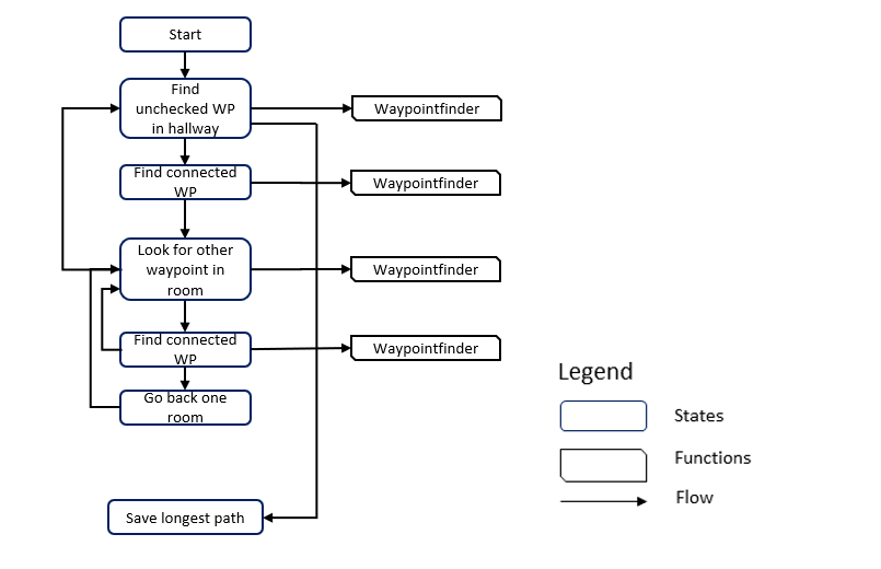
After Parking, Pico has to start searching the object. The following hint is given on the location of the object, The object is located in the room that's connected with the hallway through the highest number of doors. A program has been written that determines the room that's furthest away from the hallway. The function find_longest_path, starts by looking at the first way-point in the hallway and finds its connected way-point. the program then looks at which room the connected way-point is located and looks if there any other way-points if there are other way-points then for each of those way-points, the function finds the connected way-points and again looks for other way-points. This is repeated until no more unused way-points can be found. The program then saves the longest path it could find. The function then repeats this for all way-points in the hallway. When all way-points in the hallway are used, the program saves the longest path and the room number that the path leads to. This path consists of an array of consecutive way-points that lead to the room. This information is then fed to the function drive_to_room. A flow diagram of the function is shown below.
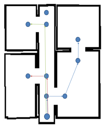
In the image below, a visual representation of the function is given for the hospital challenge map.
In the provided map, 3 paths can be found from the hallway. The first path (blue) connects 4 way-points and crosses 2 doors. The second path (red) connects 2 way-points and crosses 1 door. The last path (green) connects 2 way-points and crosses 1 door. The program then returns the path with the most door crossings. In this case this is the blue path.
In the snippets section at the end of this document, the written code for the functions find_path and find_longest_path can be found.
Driving to a room
When Pico has determined where the object is expected to be using the given hint, the function drive_to_room is given the path derived by the find_longest_path function and starts driving to the first way-point in the input array. When Pico has reached the point, it starts driving the second way-point. this is repeated until the last way-point in the array. when the last way-point is reached, the object detection function is called.
Find the object
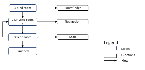
The last part of the assignment consists of finding the newly placed object. Although the functionality was not implemented yet, as was done for mapping the hospital, we already thought of a possible implementation of the functions, as can be seen in the figure above.
Step 1 (State 1):
In the first state the find_longest_path function is called, which determine the most likely rooms the object to be in.
Step 2 (State 2):
After the room order is determined, Pico starts driving to the rooms where the object is most likely in.
Step 3 (State 3):
When arrived in the room, Pico start scanning the room and compares the laser data found with the original mapping. When too much deviations are found beyond the wall, the object is found and the next state is reached. If nothing is found, Pico returns to the previous state and drives to next most likely room for the object to be in.
Modified Split and Merge Algorithm
For the detecting the features first it is essential to find out the number of sections in the surrounding. A section comprises a continuous set of data points. A section ends when the distance between consecutive data points exceeds a threshold value. In this case, it is 0.5. In the function that is made, the section details are verified by returning the indexes of the beginning and end section details into separate vectors. The index details are further used to determine the number of sections. The beginning and end details of each section is used in the split and merge algorithm to find the corners and ultimately return a 2 dimensional vector in which each row corresponds to each section and each column has elements which are of a structure type that has the x and y coordinate details, whether itś an intermediate point/ corner and if itś an exit corner or not.
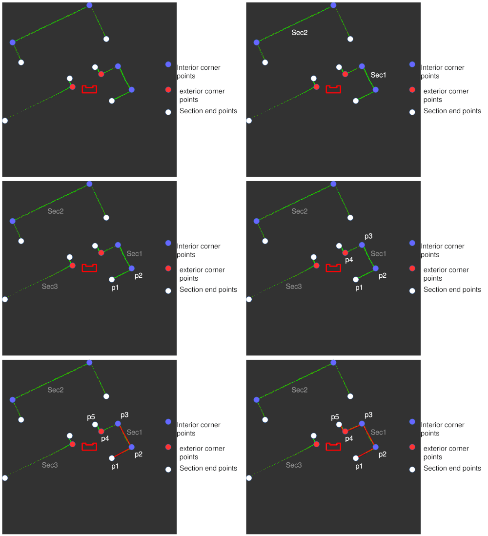
In order to generate the Map, it is essential to detect the features. This is attained using a split and merge algorithm. The basic idea of the split and merge algorithm is as follows if the endpoint and the starting point of the section are known, it fits a line between these two points and evaluates the distance of each point from this line. The point that is at a maximum distance from this line, greater than the threshold set for it being part of a wall, would be marked as corner point1, and a boolean would mark it as false for a corner point( true for intermediate point). If not, it would be identified as a wall. Now the program searches for any more corners between the starting point and the corner point1 and in between the corner point 1 and the exit point. If it finds more corner points it returns the details of these corner points and repeats until only wall segments are identified. For a section, the function ultimately returns the initial point, corner1, corner2 ... corner#n, the endpoint of the section as each row.
Algorithm
The Modified split and merge algorithm works in the following sequence:
- The starting node = Section beginning point, ending node is the section ending point.
- Line is fitted between these points and distance to each point in between is found.
- distance of each point inbetween from the fitted line is determined with the equation given below.
dist = abs( a*x+ b*y + c )/ sqrt( a²+ b² )

a = (yi - ye)/(xi - xe)

b = -1

c= (xi*ye - xe*yi)/(xi - xe)
- Check is all distances are within the threshhold.( here threshhold was tuned to 0.1 considering the fact that the wall thickness is 20 cm.
 if (distance < threshold )

Return the initial and end point with flag as true indicating that itś a wall.

else fit lines line between the initial point - cornerpoint found and the exit - corner point and search for more corners.

If all wall segments are identified with no more corners, return for the current section, the initial point, corner 1, corner 2 ... etc end point in sequence.

goto the next section, follow the same steps until the last section.
For illustration of the modified split and merge algorithm refer the sequence generated below. The threshold length mentioned here is the length for the point separated from the wall to be categorized as not a wall.
The feature depends on laser data as input, the data on reading the CSV file showed several data points as Nan( not a number). These are eliminated from the section by filtering the laser data.
- Separate structure to characterize the points(Marker Allocation)
Every point that has been detected is a structure of the following form.
- x coordinate
- y coordinate
- bool, true if it's an intermediate point, false if a corner
- bool, true if it's an exit corner
Characterizing the corners found
- Distinguishing between exterior corners and interior corners.
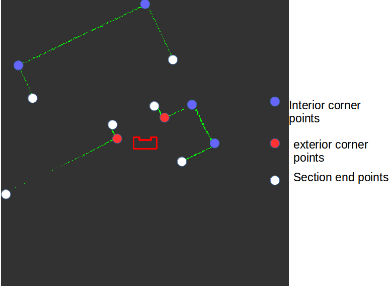
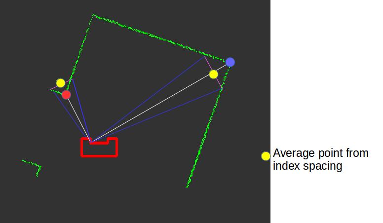
In order to distinguish between interior corner points and exterior points the following characterisation is made using the MARKERALLOCATION function. A tuning parameter(INDEX) is considered and datapoints with indices before and after the detected corner point are taken and the average of both the indices are considered. If the length of this point to PICO is more than that of the length of the corner point till PICO then itś an exterior corner point, else its an interior corner point.
- Identifying the exit points
The main criteria that was considered for an exit point to be a door is to identify that the distance between the exit point and the next immediate point in the laser range to be within the range of 0.5-1m, except for the last point in the section. If the criteria is satisfied, then the flag for the point is returned with an index of true. This can also be seen in the debugger that has been attached alongside. Only one for the points is identified with an exit corner index.The next immediate point which is at the shortest distance is found.
Test results
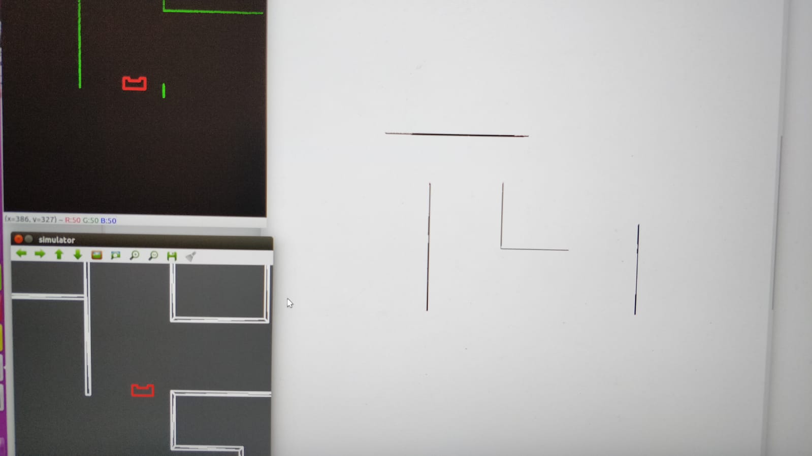
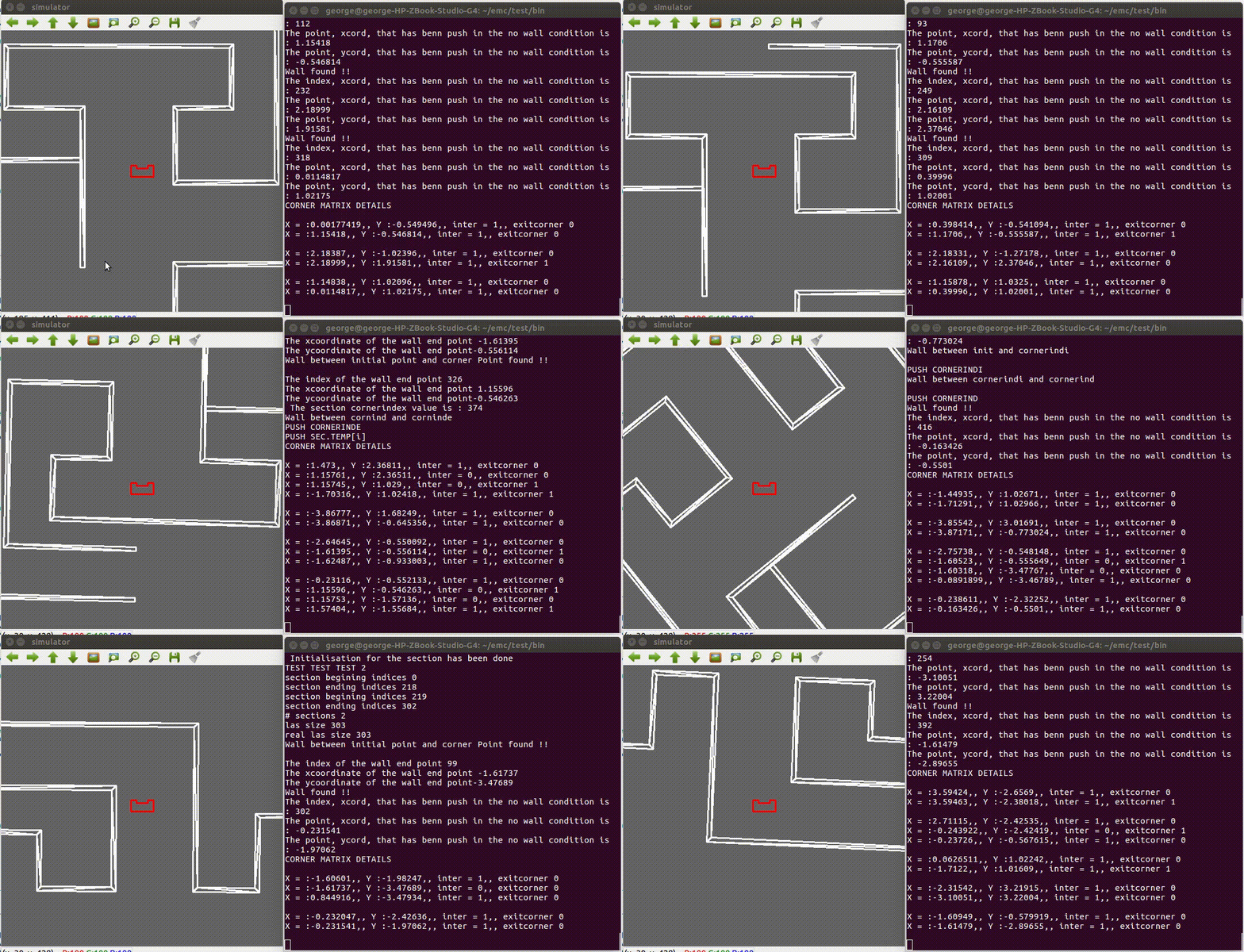
The simulation was performed on the PICO simulator by changing the threshold values do that all the features of the map are identified correctly. The results are depicted below.
From the simulation test results for split and merge algorithm it was possible to adequately determine the corners, however, in real world testing certain features at distances where the density for laser data points are less was missing. This was rectified by adjusting the threshold so that even less dense points are connected together as sections.
Debugging interface
The above interface was used to debug the modified split and merge algorithm. It gives real time values that are detected as corner/ intermediate points and on whether they are exit or not( from the bool flag). As PICO moves through the map it dynamically gives out the point which can be verified from the map used for in the PICO simulator.
The interface gives real time details of each section under CORNER MATRIX DETAILS. The details are mentioned for each section identified in the anti-clockwise direction with respect to PICO. A span angle of 180 degree is considered for each scan. Note that all end points of a section are identified as intermediate points.
Limitations and solutions
- Missing corners case .
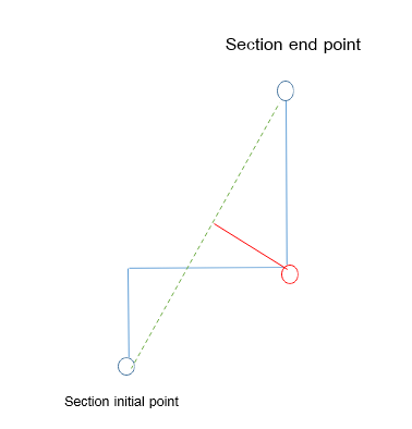
As shown in the above figure, for a general split and merge algorithm if the index of the first corner that is detected is after another corner point, it would update the initial point to the corner found and miss it. Also, to resolve this it would be required to run the algorithm with the endpoint to the initial point to identify the missed corners. Followed by which a separate function would have been needed in order to arrange them in sequence. These requirements are implicitly carried out in the modified split and merge algorithm.
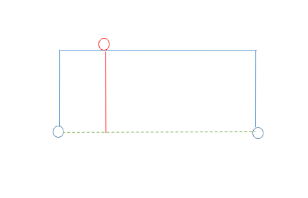
- Fitted line being a parallel case
Another major drawback faced was if the line fitted between the starting and end node of a section is searching for a corner point in a line thatś formed by two corner points which is parallel to the initial fitted line.
In this case, the corner is identified as a point on the line to which the fitted line is parallel. In this case, for the new algorithm, it checks for more corners between the corner initially found and the start point and as well as between the corner point and the endpoint. Two other corners are found on fitting. On connecting these corners the first corner would lie on a line connecting the two corners found. Hence the first corner would lie on a line.
Mapping the world
Linking corner data together
With the data from the feature detection the program can determine what the world around PICO looks like. This data can is used to create a map of the world. The feature detection returns the begin and end points of all walls, including the corners it detects between the begin and end points. The feature detection always returns these values in sequence, so it is known that the first returned point is connected to the second point and the second point in the section is connected to the third point in the section, this is illustrated in figure 7
This knowledge is saved in the world model. All these marker points are referenced against the already saved markers and saved if not saved previously. The knowledge of which markers are connected is also saved. Because the markers in a section will always be put out in the same order it can be deduced which corner markers are connected to each other. Intermediate points are not saved if they are not connected to a corner marker.
Generating the map
The map is made by drawing lines between saved corner markers and its connected markers. This map is saved with the help of opencv in a structure of 3000 by 3000 points. Walls are drawn as black lines. Markers also shown in the map with color coded points for debug purposes. Markers are only saved if they are corner markers or connected to a corner marker. So if a section consists of two intermediate points they will not be saved into the world model. The information which these markers represent is however still very valuable for localization, because it indicates there is a wall between those two points. This is why when a section of two intermediate points is detected, a line will be immediately be drawn in the map, making sure that the localization can use this information without saving the markers themselves.
Linking Exit markers
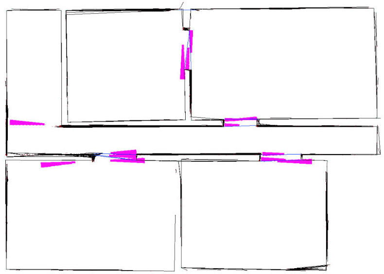
A doorway between rooms is simply put an open space between walls. The end of those walls are indicated with exit markers. However, the exit markers need to be linked together to represent a doorway. To link those exit corners, first the connected markers are checked. The exit marker should be connected to one regular corner marker and either another exit marker or intermediate marker. By determining the direction from corner marker to exit marker, the approximate angle can be determined where the accompanying exit marker is located on the map. A closest point to the exit marker is searched for within a cone. The approximated direction determined from the corner marker and exit marker is used as the center of the cone. Between the distance of 0.5 meter and 1.5 meter the algorithm searches for the closest point, as this is the minimal and maximal specified width of a doorway. If a closest point is found it will be referenced with all saved markers. If the difference in position between the found point and marker are small enough, approximately 0.1 meter, they will be linked. The correct functioning of this program is verified by drawing these cones and drawing blue lines between the linked exit markers. The result can be seen in figure 8. When these exit markers are linked they can be used to create way points to navigate the world.
Localization
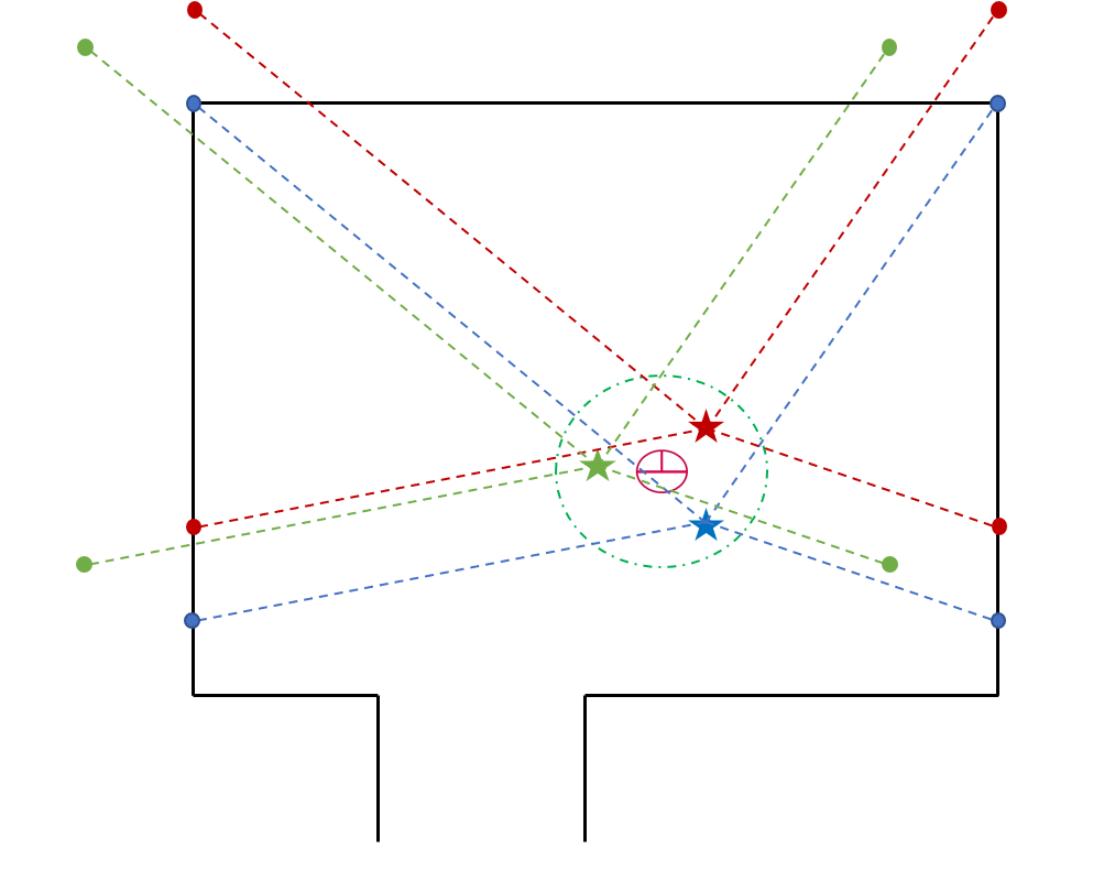
To localize PICO in the world the current laser data is referenced against the known world, the map. To help localize PICO the change in odometry is used. This gives an indication of where PICO will be. It is however not feasible to do localization purely on odometry due to the fact that wheels can slip, making it unreliable data over long periods of time. The laser data is converted from polar coordinates to cartesian and fitted on the map with varying hypothetical positions on the map, visualized in figure 9. These hypothetical positions are slight variations in angle, x and y on top of the change in odometry.
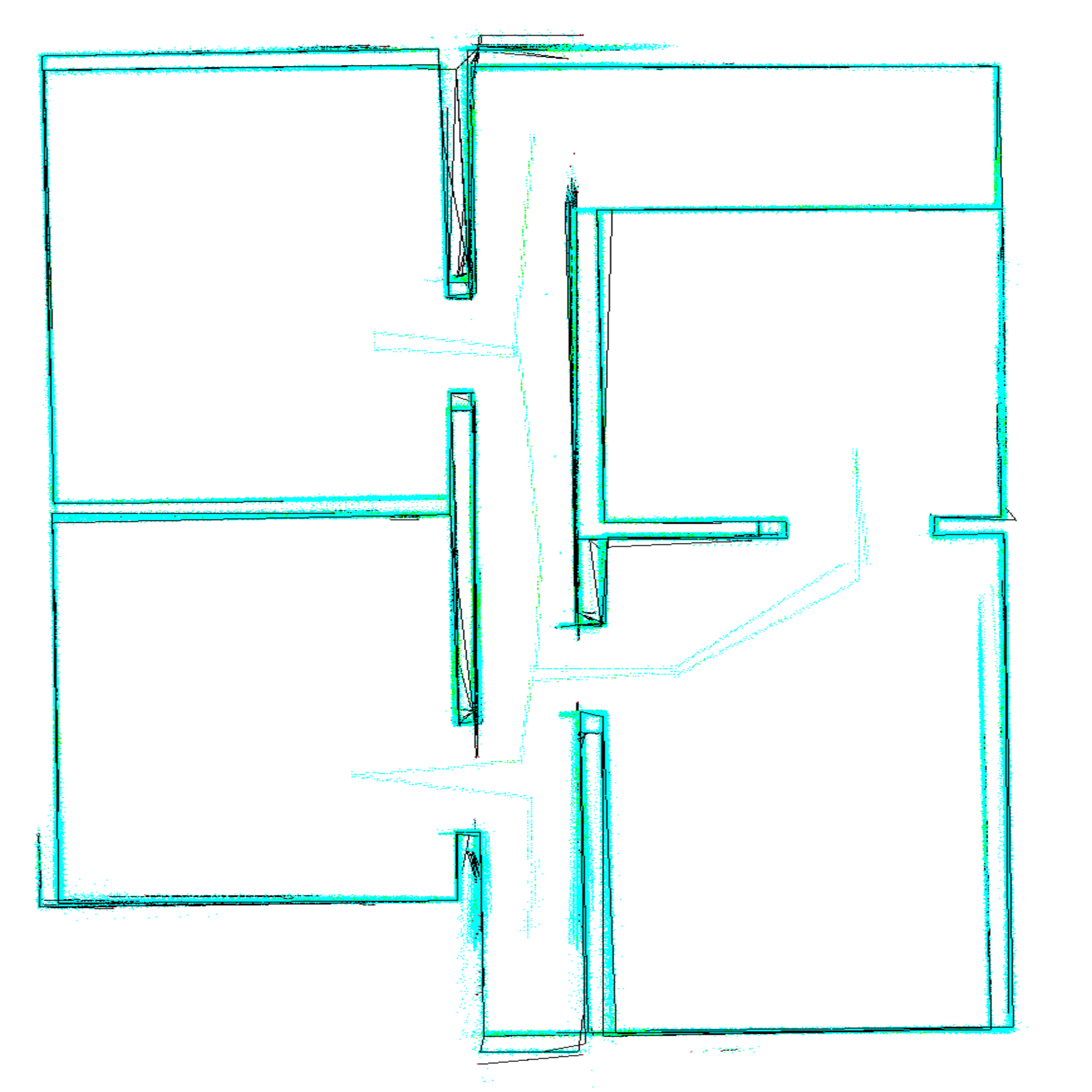
The quality of the fit is expressed with a number, the higher the number, the better the fit. This number is calculated by the number of points in the map, and their proximity, to a laser data point. The closer the point of the map to the laser point, the more points are added to the quality of the fit. Only a fraction of the laser data points are used for the localization because it is accurate enough and comparing more data would require more processing power, by which the program would slow down. In the end, the hypothetical position of PICO with the best fit will be stored as PICO's current position. To test the proper working of this algorithm the best laser fits are drawn alongside the map. Additionally, all the current calculated positions of PICO are drawn on the map, showing the path it has driven. This is shown in figure 10. The figure shows the simultaneous mapping and localization after implementation.
Simulation in hospital Map
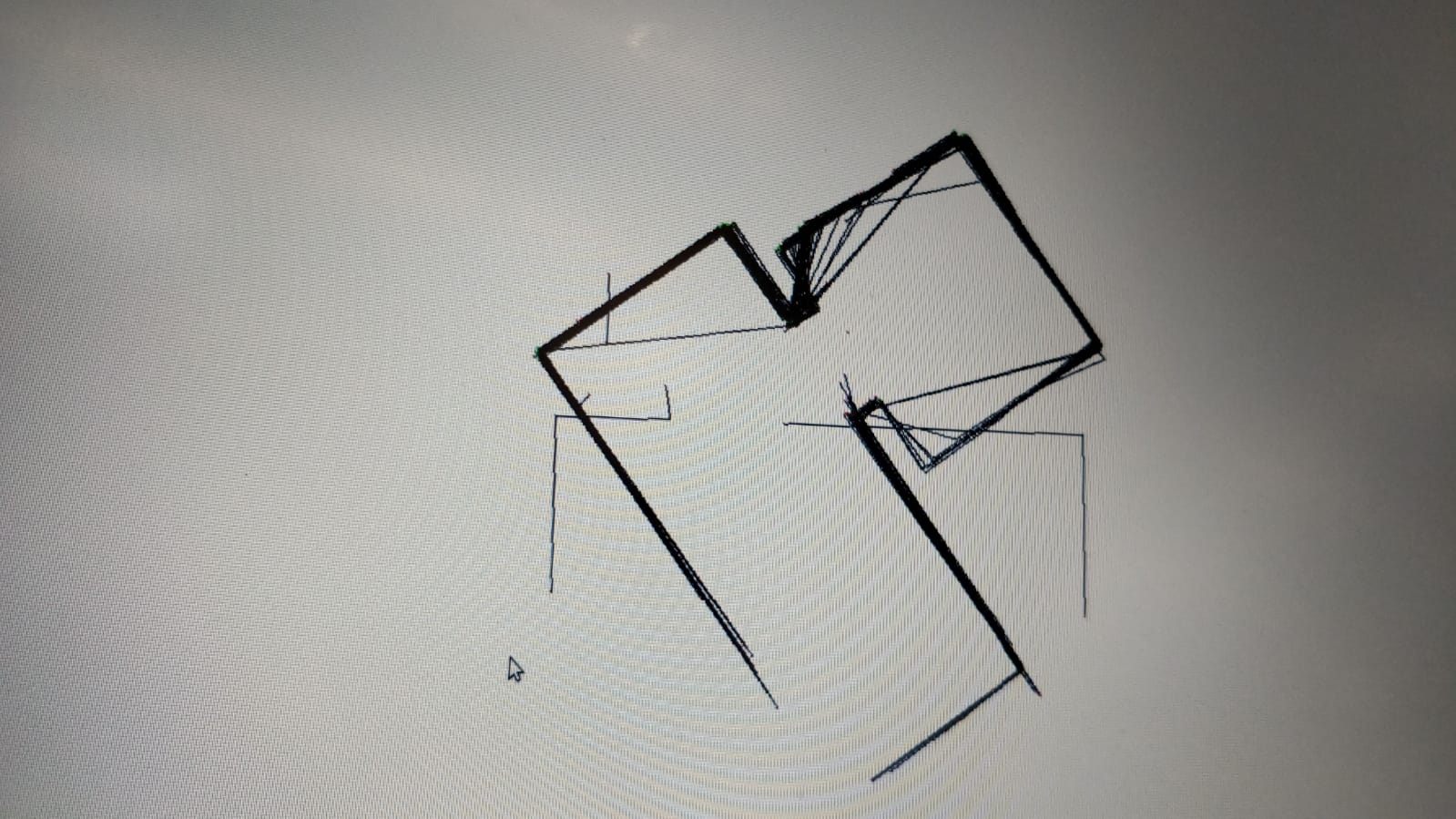
Map generated at the Hospital Challenge
During the challenge PICO did not manage to map the complete hospital. A problem occurred whereby the feature detection did not assign exit markers the correct value, which made it impossible to link exit markers and create waypoints. This is why PICO did a scan only from two points on the map. The map itself looks like we expect it to. The distance criteria not being met in real time due to excessive noise is the speculated reason. by adjusting the threshold properly this problem could be corrected.
Recomendations
- The function used for the feature detection could be made more robust to ensure it will work properly all the time, for now there are some quick fixes present.
- Due to time constraints there were deviations from the planned interface, for a more compartmentalized working this could be improved upon.
- The high level functions were not working properly, these should be finished and tested for the a program that can complete the hospital competition.
- It could be implemented that the program automatically sets the size of the laser array it should use, now it is hardcoded and may lead to segmentation errors if not handled properly.
- The occurrence of diagonal walls when mapping on the real robot should be investigated, this does not seem to happen in the simulation. It can be that the source of the problem lays with the feature detection.
