This Wiki describes the development and implementation process of software which can control Pico and help him to find the exit of a maze. Pico is a driving robot which has a Laser Range finder (LRF) sensor to view the world. It has an omni-base from which odometry measurements are available, unfortunately these measurements are prone to errors. The LRF can be compared to eyes of a human and the odometry to proprioception we have to sense where our limbs are. The only thing Pico is missing is the equivalent to a brain, the autonomous software which is to be developed. Unlike many other implementations seen this year, an intelligent way of solving is used instead of following a wall.

TODO

Iedereen: eigen deel
Matthijs: evaluatie corridor challenge
Joeri: evaluatie maze challenge
Joep: maze challenge architectuur / intro
Joeri/Iedereen: recommendation (Joeri hoofdverantwoordelijk)

Sil is voorstander om de minutes te verwijderen, aangezien er maar twee staan. (of deze moeten aangevuld worden ik heb iig geen notulen gemaakt).

Group Members

Name:	Report name:	Student id:
Matthijs van der Burgh	M.F.B. van der Burgh	0771381
Joep Linssen	J.M.H.G.H. Linssen	0815502
Sil Schouten	S. Schouten	0821521
Daniël Pijnenborg	D.H.G. Pijnenborg	0821583
Rens Slenders	R. Slenders	1028611
Joeri Roelofs	J. Roelofs	1029491
Yanick Douven	Y.G.M. Douven	Tutor

Minutes

Minutes of team meetings are available here: [1]

Initial design

The initial design can also be found in File:Initial-design-document.pdf

Introduction: The goal of this project is to autonomously solve a maze with a robot (PICO) as fast as possible. The robot has sensors, actuators and a computer on board to navigate through the maze. The computer runs on Linux 14.04 and the program language used for the software is C++. In this section the initial design is discussed, which consist of the requirements, functions, components, specifications and interfaces. This design will be used to build structured software and define required interfaces.

Requirements: To solve the maze problem the following are required

Finding the exit
Finding and opening the door
Avoiding obstacles at all times
The maze should be solved within 5 min
All tasks must be executed autonomously
The system should work on any maze
The robot mustn't get trapped in loops

Functions: The functions which have to be implemented are subdivided into the different contexts. Motion functions describe how the software gets input from and supplies output to PICO. Skill functions describe how different skills are executed in the software. Lastly Task functions implement task scheduling.

The motion functions have been determined as:

Basic actuation Give PICO the ability to move around and rotate
Getting information Receive information from LRF and odometry sensors.
Opening door Make a sound to open door.

The more advanced skill functions are:

Mapping Use information from ”Get information” to determine and save a map of the environment. This creates the world model for PICO.
Localisation Determine where PICO is located in the map created in ”Mapping”. This will most likely be implemented in the same function.
Object avoidance Use current LRF data to make sure PICO does never hit a wall.
Maze solving Use the map in combination with current and previous locations within the map to determine a route out of the maze.
Door and exit detection Using the map to detect if possible doors have been found and if PICO has finished the maze.

The task control implements switching between the following tasks:

Map making Done throughout the challenge to improve current map.
Finding doors Done in first stage of the challenge when no door has been found yet
Finding the exit Once a door has been found and opened the task is to go through the door and finish the challenge.

Software architechture pre-corridor

The initial design can be put into a diagram, which is shown in Fig: figfigfigfigfigfigfigfigfigfigfigfigfigfigfigfigfigfig. Below the diagram a short recap of the skill, world model and task contexts are given, in order of execution.

Software architecture before corridor challenge

SLAM

The slam algorithm uses the raw odometry and laser data and processes this into a robot pose and world features. The robot pose is defined as the current position and rotation of Pico with respect to the initial pose of Pic. Features are defined as re-observable landmarks, for example corners of walls, and are saved as locations with respect to the initial pose of Pico. A possible method of SLAM is EKF SLAM, but many different types of SLAM exist.

After evaluating multiple SLAM algorithms, it has been decided that EKF SLAM fits bests with the problem. The reason for this choice is that it works well in circumstances where there are clear landmarks, in our case corners, these landmarks can be used in primitive detection as well. It is also effective for problems of moderate size, the data size will not become huge and slow to process for a few hundred landmarks.

World model

The world model is a data structure that holds the detected features, primitives and pose of the robot. It takes feature and pose data from the SLAM algorithm this information is used by primitive detection to find primitives within the world model. Primitives are locations where a major change of movement direction is possible, a point where a decision has to be made.

The data in the world model is used by the state machine and maze solver to solve the maze challenge. Note that the world model does not do any data processing itself, it is merely a container of data.

State machine

Solving the maze is done in three states:

Find door
In this state the maze solver will have to detect if a possible door is near Pico, if so the state is changed to Open door.
Open door
When a possible door has been found the bell is to be rang, after which it has to be checked if the door opened. There are two possible outcomes, either there was a door, which opened, or there was no door. In the first case state changes to Find exit, else the state reverts back to Find door
Find exit
In the find exit state Pico does not search for doors anymore and has to detect if the exit is crossed in which case Pico has to stop.

Maze solver

The maze solver implements a maze solving algorithm that is able to cope with loops in a maze, for example Trémaux. It takes primitive and pose data from the world model. If Pico is within range of a primitive, a decision is made in which direction to move next and sends this data to the driving skill.

Driving

In the driving skill a driving strategy is to be implemented which is able to avoid obstacles while driving in a set direction, taken from the maze solver. Avoiding obstacles means that laser data is required to measure distances to objects in the world.

For the driving skill the best method was chosen to be a potential field method would be the best choice. Correct implementation makes sure Pico will never hit a wall while driving towards a desired location. A downside of this method is that Pico might get stuck if there a wrong decision is made.

Corridor challenge

Software architecture post-corridor

After the corridor challenge it was decided to take a slightly different approach on the SLAM algorithm and split it into SLAM for localisation and feature detection. This is change has been made since SLAM is already implemented and tested within ROS and known to be robust, and therefore focus can be placed on other crucial tasks as primitive detection.

Maze challenge

General toolset

A distinction is made between skills, which are divided in classes, and toolset functions, which implement supporting functionality. Some of these functions help cope with the non-ideality of the real-world, for example in the ideal situation Pico is placed aligned with the maze correctly every time, laser data is noise free and odometry data starts at 0 everytime. Violations of these situations have to be handled, and preferably only at one point in the code; this provides clarity and, most importantly, negates the situation where two modules would operate on different sets of data, while they should not.

Initialisation

The Maze Solver relies on the directions from the Primitive Detection being correct in the world frame: NORTH, EAST, SOUTH and WEST with respect to the initial rotation of the robot have to actually represent this. Furthermore, since the architecture requires that a new Decision Point can be found by driving in one of these cardinal directions. This adds the requirement of the robot being initialised perpendicular to a wall. Since all corners are approximately right angled this results in available directions at every Decision Point corresponding to the actual NORTH, EAST, SOUTH and WEST.

Solving this problem is fairly straight forward using Feature Detection. From the first two features, which are always in the same section, the angle between the two points is calculated. This angle is then used to turn Pico such that is in alignment with it. This is repeated until the angle is within a threshold of approximately 3 degrees. This process is shown in simulation in Fig. figfigfigfigfigfigfigfigfigfigfigfigfigfigfigfigfigfigfigfig

After aligning with a wall the first decision is made according to a laser measurement which measures for open directions in the starting position. Finally the starting pose of the mapping is set to the aligned pose, which will be used to retrieve pose data at different locations.

Shadow point filtering

Using the Laser Range Finder in practise raises a problem when scanning an ending wall: shadow points appear. They are ghost measurements, placed at an arbitrary distance behind the wall, but always at exactly the angle to the ending, and are caused by the way the sensor works (detecting reflected laser points). An example of such shadow points is depicted in Fig. figfigfigfigfigfigfigfigfigfigfigfigfigfigfigfigfigfigfigfig. Since they negatively effect the Feature Detection and Potential Field, they need to be filtered out.

The Shadow Point Filter uses one attribute of these points to discern and detect them: they commonly don't have many other measured points around them. It thus looks before and after the point in the laser data array for N steps, and checks whether less than M of these points are within a radius r of it. Is this the case, then the point is either removed or set to distance 100. Thus, we keep track of two different arrays, which each have their own usefulness for different applications.

The filter with parameters {N, M, r} = {10, 5, 0.1} applied on the previously depicted figure, is shown in Fig. figfigfigfigfigfigfigfigfigfigfigfigfigfigfigfigfigfigfigfig

Main skill set

The main skill set implements, as the name suggests, skill functions defined in the architecture.

SLAM

Because of the chosen maze-solving algorithm, a global position is required. The odometry of Pico is inaccurate and therefore useless for determining the position Pico. Localisation on the laser range finder, improves the accuracy of the position. Because the environment is unknown, SLAM, simultaneous localisation and mapping, is needed. Various SLAM algorithms are available. Choosing the correct algorithm, implementing it and tuning it can take a lot of effort, therefore Gmapping[2][3] in ROS is used. Gmapping is a implementation of a highly efficient Rao-Blackwellized particle filter.

Gmapping is only used to provide Pico with a more accurate global position than provided by the odometry. The created map is not used for detection of primitives, therefore the accuracy of the map is irrelevant.

Gmapping is combined with TF[4]. TF handles all the different coordinate frames and their transformations. TF also allows us to transform points in a specific frame to an other frame.

Feature detection

For determining the locations of decision points corner and segment features are required, from which primitive detection can generate decision points. Corner features are defined as locations where two, connected walls meet i.e. a corner, segment features are the features which are not corners which describe beginning and end points of wall segments. In Fig. figfigfigfigfigfigfigfigfigfigfigfigfigfigfig these features are shown, corner features in red and segment features in blue. Since the laser data contains values showing out-of-range data these values are set equal to 100 indicating an open section. In these out-of-range sections no features are set.

The strategy to find segment features is based on the difference between two consecutive laser points, if the difference is greater than a threshold value (set at ................) a segment is detected and both points are set as segment features. For the corner features a split and merge algorithm is applied to every segment (from an even segment feature to the next segment feature, i.e. from 0 to 1 and 2 to 3).

The split and merge algorithm works in the following sequence:

starting node = segment beginning, ending node = segment end
dx and dy are calculated between starting and ending node

distance between measured data and straight line is calculated as:

dist = abs( dy*x - dx*y + x(start)*y(start) - y(end)*x(start) )/ sqrt( dy^2 + dx^2 )

check if all points are within threshold

if(maximum distance > threshold)
ending node = index of maximum value
index of maximum value is a corner node
goto 2

done

The split and merge algorithm is also shown in Fig. figfigfigfigfigfigfigfigfigfigfigfigfigfigfig, with some resulting examples in Fig. figfigfigfigfigfigfigfigfigfigfigfigfigfigfig. This split and merge algorithm is tested in Matlab first of which executable code is provided in File:Split-and-merge-matlab.zip. As a comparison to the Matlab code also a snippet of the class implementing the algorithm is posted.

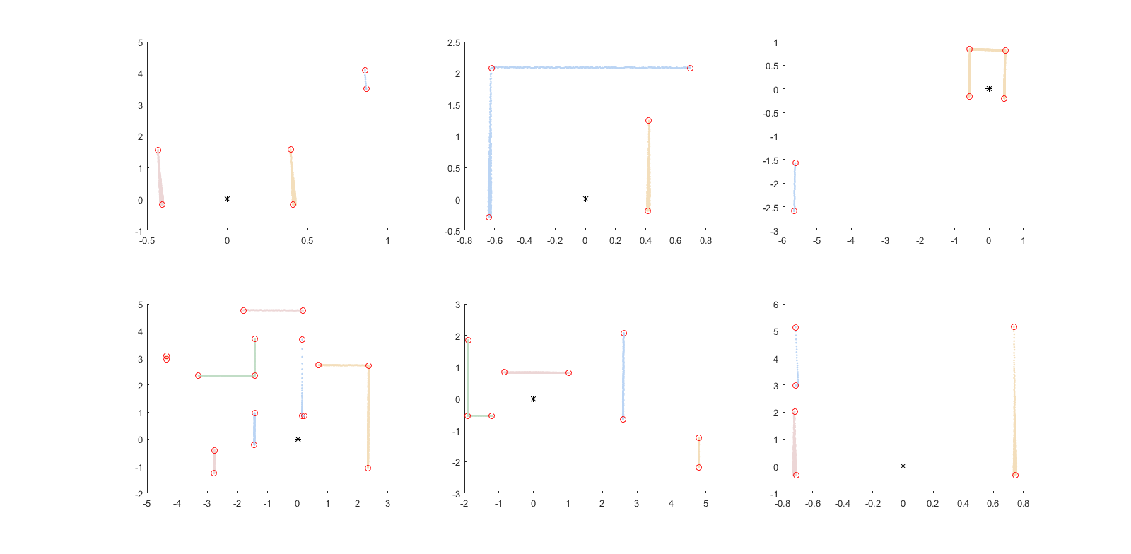
Some examples of feature detection using split and merge strategy

Dependencies: Feature detection uses laser data as its input, therefore the quality of the output depends on the accuracy of the data. If accurate data is supplied the parameters defining the strictness of the detection (i.e. the maximum allowed distance between calculated and measured lines) can be increased. This however comes with a major drawback that shadow points result in walls being split into multiple sections, as the laser data makes a jump for shadow points. To prevent this a basic shadow-point filter is implemented.

Another possible cause of error is how out of range data is handled, if this data is discarded there is are circumstances where two sections are joint together. This happens when the range before an out of range section is equal to the range after an out of range section. A result is that two sections are joint and therefore primitive detection will give a wrong output. An example of this behaviour is shown in Fig. figfigfigfigfigfigfigfigfigfigfigfigfigfigfig where the difference is shown in the corridor challenge case.

Trade offs: As mentioned in the Dependencies, the shadow point filter plays a large role in the quality of the features. In this a trade-off has to be made between filtering bad data and removing relevant information. A strict shadow point filter takes out shadow points but also leads to far-away, correct laser data being removed as well (as one laser increment leads to large range difference.

Primitives

primitives detection

The maze can be split up into primitives. A primitive is a certain part of the maze where the robot can drive in four possible directions. The four directions are north, east, south and west. These directions are with respect to the global map. In addition, each direction can contain a possible door. To determine what kind of primitive a certain part of the maze is, features and sections are used. The features location is relative to the robot, so within the local map. To check if the robot is possible to drive in one of the four directions, first the possible directions in the local map are determined. These local directions are: straight, back, right and left.

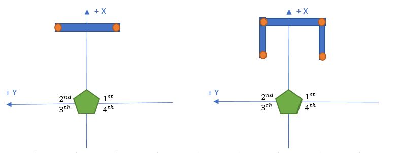
The local direction straight is possible if no section exists in front of the robot or if the section in front of the robot is more then 1.2 meters away. A section is in front of pico when it has a feature in the first and second quadrant. The straight section if also checked if it can be a possible door and is done by looking if the horizontal wall is less then 1.6 meter and if it contains two vertical walls next to the horizontal wall. In the figure below is shown an example of a straight section and a straight section with a door.

Go straight

The local direction back is always possible because it is the direction where the robot is coming from.

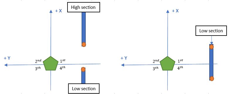
The local direction right is possible if enough space is in between two sections or a right section is 1.2 meters away. To determine the space in between two sections, a low and high section need to found. The low section has to start in the fourth quadrant and must contain a feature closest to the robot. The high section has to start in the fourth or first quadrant, must be a higher section as the low section and must contain a feature closest to the robot. In the figure below is shown an example of a high and low section with enough space in between and a right section a distance away.

take a right turn

The local direction left uses the same method as take a right turn only now the features in the second and third quarter are used.

The direction are determined locally but the maze solver needs to know them globally. the local directions are converted using the current angle of the robot into global directions.

Decison point

In addition to the global direction also the location of a primitive need to determined because this is used by the maze solver and the setpoint generator. The location of a primitive is called a decision point(DP) and has a global x and y coordinate in the map. The global x location from the robot to the DP must be exactly in the middle of a right/left turn and 0.5 meter in front of dead end or door. The global y location from the robot to the DP is zero. To get the global x and y in the map the x and y location of the robot needs to be added. To improve robustness, decision points can only be determined when the robot has a certain angle and an averaging filter is used to filter away wrong decision point.

Maze solver

The mazesolver is designed to make decisions at each primitive, it has to make decisions in such a way that it will find its way out the maze in preferably the shortest path. It also has to make sure that the robot does not get stuck in a loop.

There are multiple possible algorithms for designing a mazesolver. Since it is not know where the exit of the maze is strategies using a heuristic, like A* will not be considerd. A few options that we did consider are:

Wall follower This algorithm is very simple it always follows the wall on one side The disadvantage of this algorithm is that there is a possibility for endless loops

wallfollower path

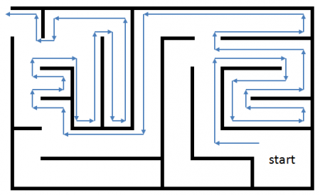
Pledge algorithm This is an extension of the wall follower algorithm, This algorithm also keeps a count of the sum of the turns to avoid obstacles.

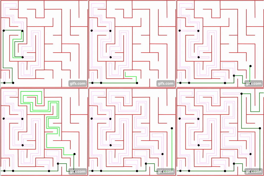
Trémaux's algorithm/ Depth-first search The Trémaux's algorithm is an algortihm that remembers the decisions made on a crossing, it uses this information to prevent it form entering the same path twice, therefor it should avoid loops.

The algorithm has the following steps:

Mark each path once, when you follow it. The marks need to be visible at both ends of the path. Therefore, if they are being made as physical marks, rather than stored as part of a computer algorithm, the same mark should be made at both ends of the path.
Never enter a path which has two marks on it.
If you arrive at a junction that has no marks (except possibly for the one on the path by which you entered), choose an arbitrary unmarked path, follow it, and mark it.
Otherwise:
- If the path you came in on has only one mark, turn around and return along that path, marking it again. In particular this case should occur whenever you reach a dead end.
- If not, choose arbitrarily one of the remaining paths with the fewest number of marks (zero if possible, else one), follow that path, and mark it.

Depth-first is a special class of the tremaux algorithm, where the solver has a preferred order of choosing paths. Its name comes from the fact that this algorithm will always explore an entire branch of a tree before going to the next one.

Breadth-first search With breadth first we will first check how many nodes there are connected to the current node and explore these in a fixed order by number, during each exploration the new connected nodes will be numbered incrementally. The biggest difference with Depth-first search is that at each node first all the options are explored before going one node deeper. https://www.youtube.com/watch?v=ec0IJsiIuWk

The wall follower algorithm is not suitable for our application since we might have loops in our maze. The Pledge algorithm however might work, but is still a relative dumb search method. The Trémaux's algorithm/depth-first is already a bit smarted since it keeps track of the intersections it has been on. This requires some memory but not an entire map of the maze, since it is simply possible to follow back the wall to the last intersection. Only the coordinates of each intersection with the explored options have to be remembered. This algorithm is better suited for our application than the breadth first algorithm since the breadth first would require the robot to drive back after each iteration while the depth-first only has to drive back on a dead end. Therefore we decided to use the depth-first algorithm for our mazesolver

Implementation

To implement the Depth-first algorithm we created a class to store the nodes at which decisions where made. Such a node would contain its position in the world frame, and the options for each of the for directions. The for directions are North, East, South and West. These are always absolute directions in the world frame.

The options for each direction are:

-1 : there is a wall in this direction
 0 : the first time I entered this node, I came from this direction.
 1 : there is a free path in this direction
 2 : there was a door in this direction
 3 : there is an exit trough here.

These were chosen in this way such that the mazesolver just can pick the direction with the highest value. After choosing a direction this direction is set to -1 in the node, this ensures that the robot will not take the same direction the next time it comes at this node. If the robot finds a node with no options to explore it will return to the previous node and explore the next option of this node. If the robot encounters a node that is already in its list but is not a parent to the previous node it will turn around and it will mark the path in that node as explored(-1). this will prevent the robot form exploring the same path twice from different directions.

To ensure the mazesolver only makes decisions when needed a separate function to call the mazesolver was created. This function checks if a new primitive really is a new primitive or that it rather is the previous primitive just shifted a bit, further it checks if we are close enough to the primitive to make a decision. Finally if there is a possible door detected this function will first call a function to check for a door and then call the mazesolver with the outcome of this function.

The door opening function simply checks the average laser distance in 3 zones left right and in front. After checking the distance it will ring the bell wait a few seconds and check again. If one of the distances has increased by a certain threshold a door has opened and the mazesolver will decide to go throughthis door.

Set-point generation

The setpoint generator provides the system with a global setpoint. This setpoint is afterwards transformed to a local setpoint. This is required, because the potential-field uses only local information. The setpoint is only a position. The rotation of the robot is handled by the potential-field.

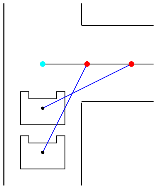
The setpoint generator places the setpoint on a straight line in direction chosen by the maze solver. To prevent Pico from touching the walls, the setpoints are always placed on a predefined distance from the center of pico. Therefore the input of the potential-field is bounded at a controllable level. The closer Pico is to the decision point the further sideways the setpoint is placed. This is implemented by constraining one coordinate to the coordinate of the decision point and the other coordinate is free to be calculated, so that the setpoint is at the desired distance. The constrained coordinate is depended of the chosen direction. This is shown in Figure. figfigfigfigfigfig.

Potential field

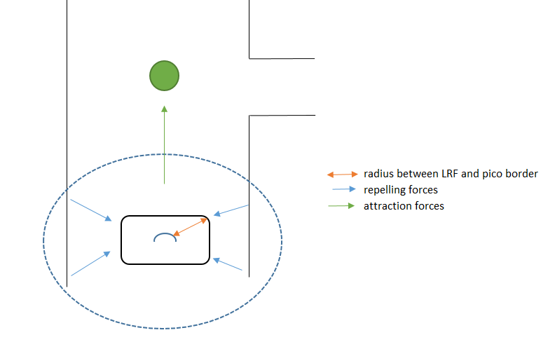
A potential-Field Algorithm is designed to make sure PICO never collides with walls. A schematic of the repelling and attraction forces is made, see figure 1… The green dot is the desired position of the robot (which is the output of the setpoint-generator), the blue dotted circle is the range of the LRF. It is not needed to use the full range of the LRF because avoiding collision is only required in close range to any walls. A range of 4 m is used.

Repelling forces

The repelling forces are calculated by the following formulas:

$[math]\displaystyle{ r_rep=-F_bad*(√((cos⁡(a)*abs(r-r_pico ))^2+(sin⁡(a)*abs(r-r_pico ))^2 ))^(-3) }[/math]$

$[math]\displaystyle{ F_r=(█(F_repx@F_repy ))=■(∑_(i=1)^n▒〖cos⁡(a[i])*r_rep 〗@∑_(i=1)^n▒〖sin⁡(a[i])*r_rep 〗) }[/math]$

r_rep is the length of the repelling force vector. a Is the angle of the laser beam in rad, r is corresponding the measured range of the laser. The measured distance is then r subtracted by r_pico the range between the borders of PICO and the LRF sensor. This is done to make sure the force goes to infinity when the robot is at collision with the wall. The laser data (a,r) is converted to(x,y), after this is done the length is calculated and this is taken to the power -3, the closer to the wall the bigger the force. This length is scaled with a factor F_bad, this factor had to be determined during tests.

Attraction force

The attraction forces are calculated by a quadratic equation:

$[math]\displaystyle{ r_att=F_good* √(((setpoint_x )^2=(setpoint_y )^2 ) ) }[/math]$

r_att is the length of the attraction force vector, setpoint_x,setpoint_y are coordinates in the body frame generator by the setpoint-generator, F_good is the tunable parameter during tests.

$[math]\displaystyle{ a_att=arctan⁡((setpoint_y)/(setpoint_x )) }[/math]$

a_att is the angle of the vector in rad.

$[math]\displaystyle{ F_a=(█(F_attx@F_atty ))=(█(cos⁡(a_att )*r_att@sin⁡(a_att )*r_att )) }[/math]$

F_a is the attraction force vector. A quadratic equation is used to increase the attraction force for set points far away. The closer to the set point the lower the attraction force.

Speed calculation

Speed is calculated based on the repelling and attraction forces. First both vectors are added to obtain a total force:

$[math]\displaystyle{ F_tot=F_a+F_r }[/math]$

F_tot is the sum of the attraction and repelling forces.

$[math]\displaystyle{ A_tot=arctan⁡(F_toty/F_totx ) }[/math]$

A_tot is the angle between the x and y component of F_tot. These parameters are converted to speed parameters:

$[math]\displaystyle{ speed=■(v_x@v_y@v_t )=■(F_tot (0)@F_tot (1)@A_tot/Anglescaling ) }[/math]$

A snipped of the potential-field class can be found here: https://gitlab.com/emc2017/group2/blob/master/src/potential-field.cpp

Files

Initial design document: File:Initial-design-document.pdf

Initial design presentation: File:Initial-design-presentation.pdf

Evaluation

Evaluation corridor challenge

Pico was able to complete the corridor challenge and delivered with a fourth place. This could have been better, if Pico did not hit the wall twice. The reason for hitting the wall has two causes, devided over the lower and upper part of the software.

Pico was able to detect the corridor early, while it was still far from the corridor. It also decided early to drive into this corridor. This does not mean that the setpoint was placed incorrectly. It was still placed in the middle of the corridor. But the setpoint attracted Pico to the right. This is where the second cause comes in play, the potential-field.

The potential-field was not tuned correctly. Especially, the radius of Pico was taken into account. This means that the Repulsive forces did not go to infinity, if Pico's sides were very close the wall. This is added afterwards and reduced touching the walls to nearly zero during the following tests.

Evaluation maze challenge

Numerous parts of the code were changed after the last test session and therefore only tested in simulation. The placement of decision points in open space was added after last test session. Another problem was the speed limit of PICO. The speed limit war reduced from 0.3 to 0.15, because this improved the primitive detection in simulation. This speed limit was to low. Due to the friction, PICO was not turning to desired orientation, which stopped Pico from driving. This was embedded in the code to make Pico straight ahead in corridors and not rotated. Besides the driving problem, the other parts of the code were working correctly. After the door one decision point was missed, and caused to code to be in a loop where it was stuck in that corner.

Solving mazes!

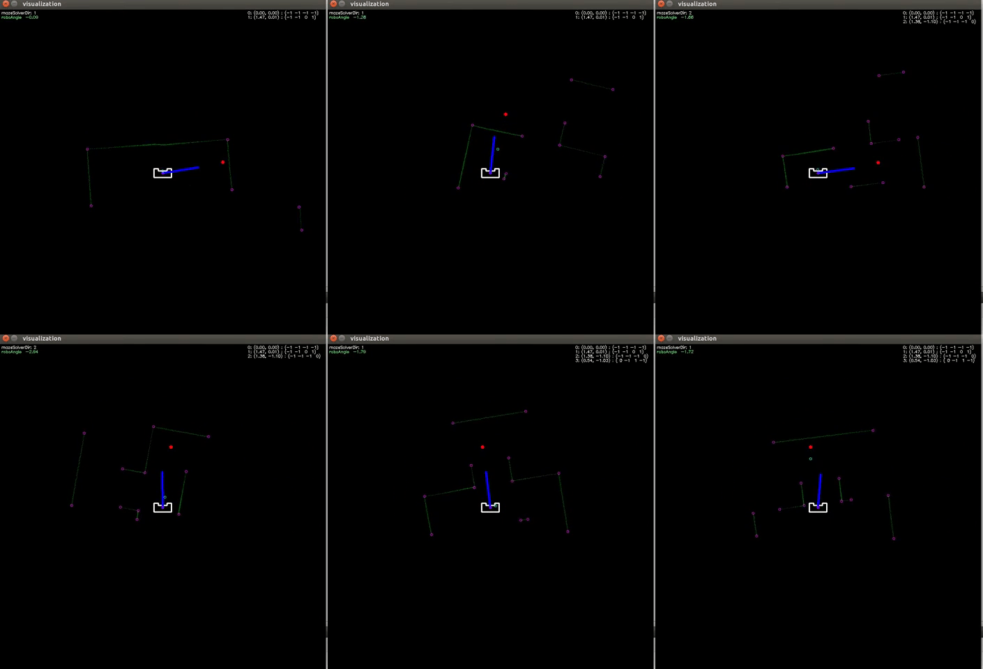
Solving the maze in simulation

The mazes of this and last year are solved by the code version which was used during the maze challenge. A short gif is shown below in where all parts of our code are working together. The red dor is the setpoint generated by the setpoint-generator, the blue line is the total force, the purple dots are the landmarks detected by the landmark detection and the blue dots are the decision points placed by the primitive detection. In the upper right corner the decision points with the directions are shown. The Upper left corner shows the chosen direction of the maze-solver and the current rotation of the robot. Whenever the Robotangle shows red the robot is in the incorrect rotation and the primitive detection is temporary disable, because it will not produce correct decision points.

Full simulation of current and last year are found here:

https://www.youtube.com/watch?v=buuI6-kGCbk

https://www.youtube.com/watch?v=6uX8d2biI_A

Embedded Motion Control 2017 Group 2

Contents

TODO

Group Members

Minutes

Initial design

Software architechture pre-corridor

SLAM

World model

State machine

Maze solver

Driving

Corridor challenge

Software architecture post-corridor

Maze challenge

General toolset

Initialisation

Shadow point filtering

Main skill set

SLAM

Feature detection

Primitives

Maze solver

Set-point generation

Potential field

Files

Evaluation

Evaluation corridor challenge

Evaluation maze challenge

Navigation menu

Embedded Motion Control 2017 Group 2

TODO

Group Members

Minutes

Initial design

Software architechture pre-corridor

SLAM

World model

State machine

Maze solver

Driving

Corridor challenge

Software architecture post-corridor

Maze challenge

General toolset

Initialisation

Shadow point filtering

Main skill set

SLAM

Feature detection

Primitives

Maze solver

Set-point generation

Potential field

Files

Evaluation

Evaluation corridor challenge

Evaluation maze challenge

Navigation menu

Search