Embedded Motion Control 2012 Group 1
Group Members
| Name: | Student id: | Email: |
| Rein Appeldoorn | 0657407 | r.p.w.appeldoorn@student.tue.nl |
| Jeroen Graafmans | 0657171 | j.a.j.graafmans@student.tue.nl |
| Bart Peeters | 0748906 | b.p.j.j.peeters@student.tue.nl |
| Ton Peters | 0662103 | t.m.c.peters@student.tue.nl |
| Scott van Venrooij | 0658912 | s.j.p.v.venrooij@student.tue.nl |
Tutor: Jos Elfring
Week 1
- Installed all required software on our computers :)
- Everybody gained some knowledge about Unix, ROS and C++.
Week 2
- Everybody gained more knowledge about Unix, ROS and C++.
- Looked at Gazebo, Rviz, Turtlebot_simulator, PR2_simulator, Jazz_robot_simulator
- Managed to create 2D map with Jazz Robot Simulator: http://www.youtube.com/watch?v=Cmh8dMrmgN0
- Made presentation of Chapter 1: Introduction, Link to the presentation: http://cstwiki.wtb.tue.nl/images/Powerpoint_Chapter_1.pdf
Week 3
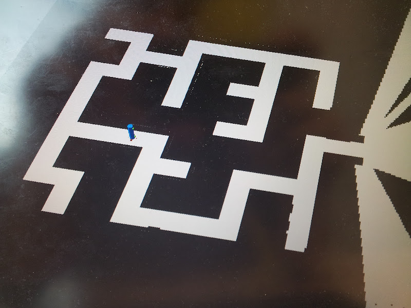
- Thought about an efficient algorithm to solve the 'maze'-problem. Depth-First-Search is proposed as a candidate algorithm.
- Started with arrow recognition using the OpenCV package.
- Started with map-processing to build up a tree of the maze which can be used by the decision algorithm.
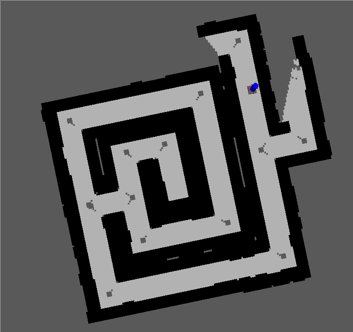
- Optimized mapping algorithm and did some processing on the map. See Figure "Optimized map"
- tarted with navigation node for autonomous navigation of the jazz
Tasks for Week 4:
- Process map
- Add markers at crossings
- Define paths between these markers for navigation
Week 4
- Arrows can be detected by camera with use of the OpenCV package.
- Robot can detect its position in a corridor with use of its laser data and can drive autonomous.
- Corner detection; extracted out of the occupancy-grid. See Figure "Corner detection".
Week 5
- Map-processing is cancelled, since the used package (hector_mapping) creates incorrect maps.
- Now working on processing the laserdata to let the Jazz drive "autonomously"
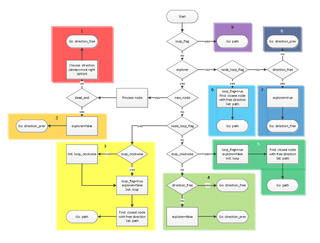
- Writing an algorithm by using depth-first-search, this algorithm obtains the kind of crossing, the position of the Robot and the angle of the Robot and sends the new direction to the Robot
Week 6
- Did tests with the real Jazz Robot; some issues were find concerning the update-rate; perhaps a new navigation strategy is needed. http://youtu.be/_g9S24xXes4
- New navigation strategy implemented. Still a couple of bugs that have to be fixed; this is for next week.
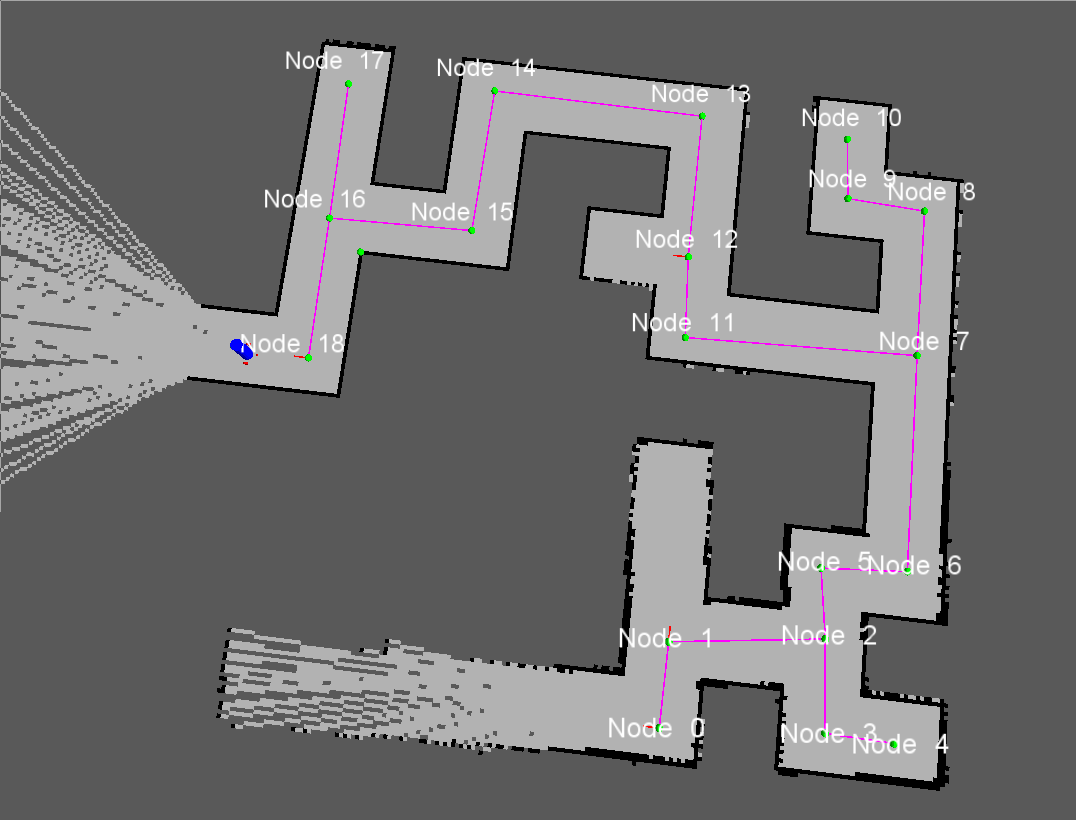
- Created a visualization-class to visualize the node-structure for better perception of the algorithm.
- Finished DFS algorithm; algorithm works now if there are no loops. http://www.youtube.com/watch?v=KSjsA6BR-Bs&feature=channel&list=UL
Tasks for Week 7:
- Debug navigation node; fix issue with no 'corridor' between 'corners'.
- Debug algorithm; try to find some errors.
- Corridor competition
- Test on real robot
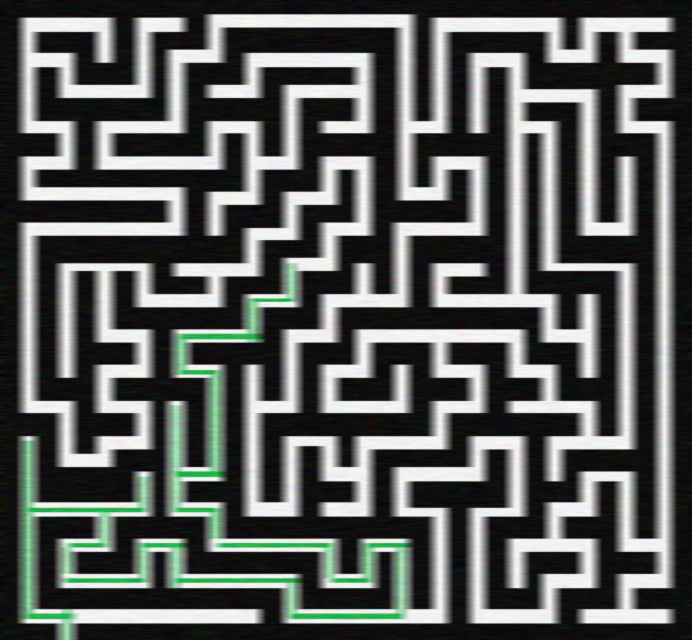
Week 7
|  |  |
Week 8
- Some adaptions on code with new simulator; result: http://www.youtube.com/watch?v=tgHOjsxDUjk&feature=plcp
The navigation node is used to steer the robot correctly in the maze. This navigating is done with use of the laser data. The laser data is first set into a certain variable. On the basis of this variable the robot can be navigated through the maze. The navigation is divided into 6 cases.
The first case is the case in which the robot is driving trough a corridor. In this case the robot is kept in the middle of the corridor by checking and adjusting its angle with respect to the walls of the corridors. While driving trough it is constantly checked whether a corner of any type or a dead end can be recognized. Whenever a corner is recognized, the navigation switches to case 2.
In case 2 the recognized corner or dead end is labeled as one of seven possible corner-types. This corner-type can be a corner left or right, one of three possible T-junctions, a cross-over or a dead end. These corner-types all get a number to identify them easily:
0. Dead end
1. Corner right
2. Corner left
3. T-junction middle (means the robot approaches for the middle)
4. T-junction left (means the robot approaches for the left)
5. T-junction right (means the robot approaches for the right)
6. Cross-over
This corner-type is now published together with the coordinates of the center of this corner-type. The coordinates of the center of the corner-type, also called the coordinates of the node, can be retrieved by processing the coordinates retrieved from the map topic, published by the hector_mapping node. Now the algorithm node processes this corner-type and at its turn publish the direction the robot should go. If the corner-type is 0 (dead end), the navigation node will still publish this type and the coordinates of the node, but then the navigation directly switches to case 6. Once the direction in which the robot should go, is received, the navigation switches to case 3.

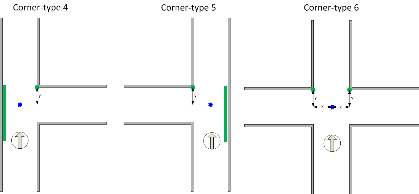
In case 3 the robot drives to the middle of the corner-type. To get to the middle of a corner the robot uses different points with respect to which it gets to the middle. If the corner is of a type in which the robot would drive into a wall if it would not make the corner (type 1, 2 and 3) it uses the distance to the wall to know when to stop driving forward. If this distance is half the distance of a corridor, the robot has reached the middle. If the corner is of type 1 (corner right), the robot uses its laser data on the left, to keep the right distance from the walls it is driving parallel to, while driving to the middle of the corner. With a corner of type 2 (corner left) it does the same, only with the laser data on the right. A type 3 corner (T-junction middle) is the only corner-type in which the robot does not have any points with respect to which it can stay in the middle, while driving forward. In Figure “Corner-type 1, 2, 3” the corner-types 1, 2, 3 can be seen, with in green the laser data or points with respect to which the robot drives to the middle of the corner.
If the corner is of type 4, 5 or 6 the robot uses the distance to the 90 degrees corners to know when to stop driving forward. When the y-distance (distance in the way the robot is driving) is half the distance of a corridor, it has reached the middle. With corners of type 4 and 5 the robot uses its right or left laser data the same way as it uses it when driving to the middle of a corner of type 1 and 2, to stay in the middle while driving forward. With a corner of type 6 the robot uses the x-distance to the 90 degrees corners to stay in the middle while driving forward. When the robot has reached the middle, the navigation switches to case 4. In Figure “Corner-type 4, 5, 6” the corner-types 4, 5, 6 can be seen, with in green the laser data or points with respect to which the robot drives to the middle of the corner.
In case 4 the robot makes a turn or does nothing. This is dependant of the direction in which the robot has to go. If the algorithm node publishes as direction to go straight ahead, the robot will not do anything in case 4 and will immediately switch to case 5. On the other hand, if the algorithm publishes to go to the left or right, the robot will make a turn of +(1/2)π radials or -(1/2)π radials respectively. After the turn is completed, the navigation switches to case 5.
In case 5 the robot starts driving forward again until it reaches the corridor. When the corridor is reached, the navigation switches back to case 1.
Case 6 is the case in which the navigation goes, when the robot is driving towards a dead end. In this case only direction is possible and that is backwards. So after driving to center of the dead end, which is at half the distance of a corridor of the dead end, the robot will make a turn of π radials. After the turn is completed, the navigation switches back to case 1.
