Mobile Robot Control 2023 Wall-E
Group members:
| Name | student ID |
|---|---|
| Lars Blommers | 1455893 |
| Joris Bongers | 1446193 |
| Erick Hoogstrate | 1455176 |
| Noortje Hagelaars | 1367846 |
| Merlijn van Duijn | 1323385 |
| Sjoerd van der Velden | 1375229 |
Design presentation
The file for the design presentation can be found here:File:Design Presentation Group WallE.pdf
Introduction
For the last several years, restaurants have suffered from a labor shortage. Everywhere around the country restaurants workers are subjected to a heavy workload with no end in sight. In an attempt to resolve this problem, we set out as a group of 6 students to design an algorithm for a robot that can deliver orders to tables. In the span of 10 weeks, we learned all about software design and autonomous robots and immediately put our new knowledge to work in exercises and challenges.
On this wiki page the following aspects of the project are discussed. First, the strategy with regards to the restaurant challenge is discussed. Next, the software architecture and robustness is explained. Finally, the results are evaluated and a conclusion is drawn.
State flow diagram
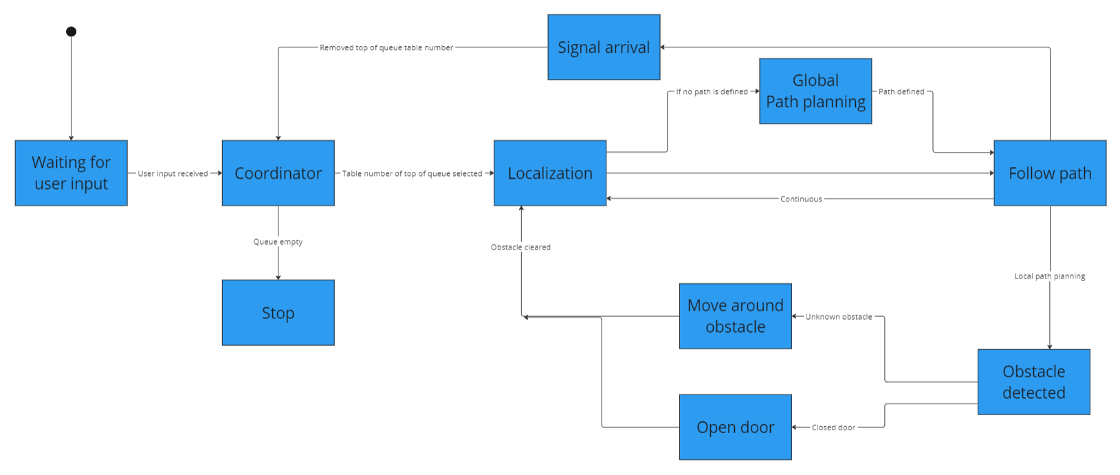
The state flow diagram, a type of behavioural diagram, shows the design of the discrete control within the system. They graphically represent finite state machines.
The state flow diagram is a representation of what the blocks in code should do, when a certain input is received or a certain object is detected. The main aspects are worked into this, including the local and global path planning, obstacle avoidance and localization. This gives a rough idea of how the robot should behave.
Data flow diagram
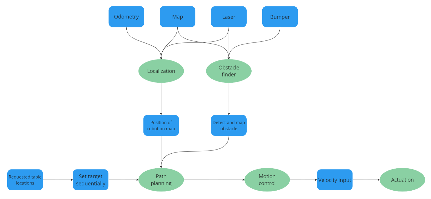
The data flow diagram shows a structured analysis which gives insights into the origin of the data and interfaces between processes. The diagram consists of data, representing the information, process, which is a functional component with inputs and outputs, and lastly the flow, which specifies an input/output relation between the process and the data.
The data flow diagram uses all data available and the flows point to the appropriate processes in order to execute those parts accordingly with the received data.
Strategy description Restaurant challenge JORIS
Below a the general strategy is mentioned, which is used by the group to get a idea of the tasks of the robot and the algorithms that needs to be used. Furhter details about the final algoritms will be discussed in the other sections below.
1. Initialization:
- Receive the list of tables to visit in the correct order.
- Load the provided map of the restaurant.
2. Localization and Mapping:
- Use the particle filter as localization algorithm to estimate the robot's position within the restaurant environment.
- Process the LiDAR data to build and update a map of the environment.
3. Global Path Planning:
- Use the A* algorithm as the global path planner to generate an initial path from the robot's current position to the first table on the list. The global path consist of waypoints (nodes), which the robot has to follow
- Consider the map information, such as walls, doors, and tables, to plan a collision-free path. Doors can be open or closed, the robot should now where the doors are to avoid local path planning at this location when the door is closed. The robot should make a sound signal to open the door.
4. Local Path Planning (Open space approach):
- Continuously check the LiDAR data, for detecting obstacles.
- If an unexpected obstacle is detected or a wall is too close, switch from global to local path planning for obstacle avoidance.
- Reassess the obstacle situation continuously and adjust the local path if needed. When using the open space approach the robot will check where the the most room is available and will drive in this direction. When an object suddenly comes too close the robot will just dogde the object.
- Reaching a safe region: Switch back to global path planning once the robot reaches a safe distance from the obstacle.
5. Switching Back to Global Path Planning:
When the decision is made to switch back to global path planning:
- The robot is slow down temporarily to ensure safety during the planning of the new path.
- Replan the global path using the current robot position and the closest node.
- Calculate the new global path as a revised sequence of waypoints to follow.
6. Table Delivery:
- Drive the robot to the first table, following the global path.
- Position the robot near the table. Make sure the robot is facing the table with a suitable range for the order delivery.
- Use a sound signal to announce the robot's arrival at the table.
- Wait for a predefined time period to ensure the delivery is complete.
- Repeat the above steps for each table on the list, following the specified order.
7. Error Handling and Replanning:
- Errors can occur due to unexpected situations, such as failed table delivery attempts. When this happens, the robot should replan to generate an alternative path or recovery strategy.
- Replan the global path considering the current robot position, remaining tables, and updated environment information.
Software Architecture Restaurant challenge
Structure of software
In the exercises during the first weeks of the course all seperate elements of the robot control like global and local path planning and localisation were treated. The challenge was then to combine all seperate functions into one executable that can be called with:
./hero_do_your_thing 2 3 4
The folder containing the main executabe file also contains the files from the A*- algorithm (global path planning), the open space approach (local path planning) and the localisation (particle filter). The executable uses multi-threading in order to run the navigation and localisation algorithms in parallel. Two threads are run simultaneously, one calling the function for navigation and one for localisation.
The navigation function first retrieves the table order as arguments and stores it in a table list variable. This table list is then used together with a table nodes list to determine the predefined node in the map that corresponds to the table. The loading of the json file containing the map parameters including the node definitions is hardcoded into the executable. The node list containing nodes that correspond to the tables that have to be visited by the robot is used in a for loop where the A*- algorithm is used to compute a path from the start till end node. For each loop in the for loop the previous end node is taken as the new starting node for the new path. Once the robot had reached the table node it will signal the customer that it has arrived with the io.speak() function. Once the robot notices an obstacle within a set range in its laser data the robot will switch from global path planning (A*- algorithm) to local path planning (Open space approach) and try to dodge the obstacle. After a set time interval the robot will use the node that is closest by to determine a new path using the A*- algorithm.
The localisation function determines the location of the robot on the map using odom data, laser data and information from a png file of the map. The particle filter estimates the current location of the robot and stores this data in a variable. A pointer pointing to the location of this variable is given as an input to the navigation function so the robot can follow the path computed by the A*- algorithm.
Global path planning MERLIJN & NOORTJE
As previously stated, the A* algorithm for global path planning provides the shortest route from a specified start node to a designated end node. In order for the A* algorithm to generate the intended path, it is necessary for the restaurant map to include nodes that connect to the desired table nodes. These nodes will serve as the basis for creating a global path.
Node definition NOORTJE
- Vector map
- Node placement
A*- algorithm
The A* algorithm is a widely recognized search algorithm that starts at a designated start node and navigates to a target end node. Each node possesses three values: 'g' represents the cost of movement from the start node to the current node, 'h' estimates the movement cost from the current node to the end node, and 'f' represents the sum of 'h' and 'g' for the current node. The 'h' value, also known as the heuristic, is determined by calculating the Euclidean distance from the current position to the end node.
When the A* function is invoked with the provided start and end nodes, the first step involves initializing the open list. This initialization involves assigning initial values (infinity, distance to the end node, and the sum of 'g' and 'h') to the 'g', 'h', and 'f' values, respectively, for each node. Additionally, the parent parameter of each node is set to None. Then the values for the start node are computed. The ‘g’, ‘h’ and ‘f’ values are zero, the Euclidean distance between start and end node, and the sum of the previous value respectively.
Following the initialization, a loop is executed, which follows a specific sequence. Initially, the node with the lowest 'f' value is determined. Next, the neighboring nodes of this selected node are added to the open list. This addition is carried out by computing the 'g', 'h', and 'f' values for the neighboring nodes and setting the parent node parameter to the current node with the lowest ‘f’ value. If a neighbor is already present in the open list, but the newly calculated 'f' value is lower than the currently saved 'f' value, the 'f' value and parent node are updated accordingly. This process continues until the node with the lowest 'f' value becomes the end node. At this point, the desired path has been found, and the code exits the loop.
Following the discovery of the path, the code enters a subsequent loop, which retraces the path from the end node to the start node using the parent node parameters. This backtracking loop enables the determination of the complete path.
The A* algorithm calculates the path to each specified table from the current node. Once the path has been established, the next step involves guiding the robot along the determined path. This task can be accomplished by utilizing the provided code from the A* assignment previously provided in this course. Particularly, the simulate_path_following function is invoked when the path has been found to let the robot follow the path.
Local path planning (Obstacle avoidance) SJOERD & JORIS
As mentioned before, the robot will switch from global to local path planning when an object is detected too close to the robot. The laser data is therefore scanned continuously. Two methods have been considered, the Artificial potential field algorithm (APF) and the open space approach. In the first subsection, the two algorithms will be compared. Thereafter, the chosen algorithm will be discussed in more detail.
Algorithm selection
- APF vs Open space
When using APF there will be a repulsion effect on objects and an attraction force on the goal. The repulsions and attractions forces are combined to obtain an artificial resulting force which indicates the motion direction of the robot. In this way, the robot will avoid obstacles and drive in the direction of the goal. The robot uses a box function where it checks the laser data around the robot in a box shape. The box is chosen such that the distance to an object to the sides of the robot is less and the distance to an object in front of the robot is more. Therefore, it will ensure that it can drive in narrow corridors. When an object is detected the robot will drive around it. when a dynamic object suddenly occurs in front of the robot, the robot will stop to avoid a collision. A video of the APF approach can be seen via the following link. https://tuenl-my.sharepoint.com/:v:/g/personal/j_bongers_student_tue_nl/EYRkNrkVgjdPu6bbLFQCorIBIDNwWcsweIXgLUfNDBrKQw?e=Pmz18h
When using the open space approach, the laser data is used to check in which direction there is the most space. Only laser data in a cone in front of the robot will be used to check for the available room. When the open space is detected, the robot will drive in this direction. Besides, the robot will dodge objects when they are located too close to the robot. (NOT SURE IN WHICH DETAIL THIS NEEDS TO BE DISCUSSED AS THIS WILL BE DONE IN next section?)
The final choice for the local path planning was open space. This decision was made by comparing the local path-planning methods in test sessions. During testing, it was concluded that the open space approach was more robust. The APF algorithm worked also fairly well, but had some problems with straight walls sometimes. Given the time and the robust open space approach, it was chosen to continue with open space.
Open space approach SJOERD
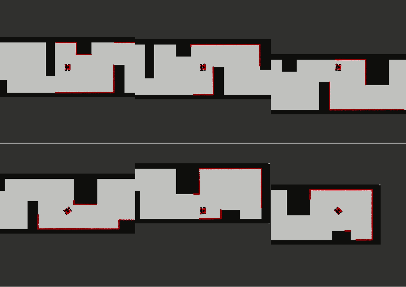
The open spaces algorithm works as a way to find the most open area for the robot to drive through. The algorithm starts once the front of the robot is measuring a distance below a threshold of for example, one meter. It works with a horizon, which is a distance that is defined as the average of the distance measured by all laser points. When comparing the laser measurements with the horizon, the algorithm searches for the largest consecutive streak of laser measurements that are larger than the horizon. Once found, it will rotate the robot to this open space and the algorithm will be completed.
Via this link a video can be seen where the open space approach works on the robot. https://tuenl-my.sharepoint.com/:v:/g/personal/j_bongers_student_tue_nl/ETw0Taaw2eNKiABZ_cSD3fEBMB7QZqVudnEAvLIGup9aWw?e=Nuhatn
-Integration with global path planning?
Localisation LARS & ERICK
Localisation is necessary to determine the location of the robot in its environment. Determining the robots location solely on data from the wheel encoders results in a wrong location due to sensor drift and slip from the wheels. Laser data, odometry data from the wheel encoders and information from the map is combined to get a better approximation of the robots current location. Localisation is done by using a particle filter algorithm. The particle filter initialises a set of particles which are possible poses of the robot on the map. A probability is assigned to each particle after which the weighted average of these particles is taken to determine the most probable pose of the robot. The cloud of particles is constantly propagated through space using the odometry data of the wheel encoders and resampled to get a more accurate approximation.
Particle initialisation
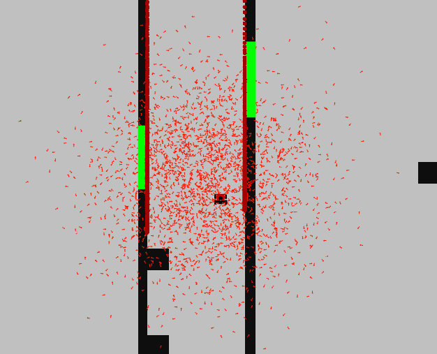
The algorithm starts by initialising the set of particles according to a certain distribution. Each particle in the set represents a hypothesis for the current pose of the robot. The particle cloud can be initiliased either through a uniform or a normal distribution. The particle initialisation through a normal distribution can be seen in the Figure on the right.
Particle propagation
Once the particles have been initialized, the algorithm proceeds with the particle propagation step. This step involves updating the positions and orientations of the particles based on the available odometry data and performing necessary frame transformations.
During propagation, the algorithm incorporates the odometry information to simulate how the robot has moved since the last update. The distance and angle traveled by the robot are estimated by adding the received odometry values, which are subject to noise, to the previous pose of each particle.
To account for frame transformations, the odometry data is first converted from the odometry frame to the robot frame. This transformation aligns the odometry information with the robot's orientation. Subsequently, the odometry data is transformed from the robot frame to the map frame, ensuring that the updated particle positions are represented correctly in the global reference frame.
By applying the necessary frame transformations and incorporating odometry data, the particle propagation step allows the algorithm to predict the new positions and orientations of the particles, taking into account the robot's motion and its relationship to the map frame. This step forms an essential part of the particle filter algorithm, enabling the estimation of the robot's pose based on its movement and odometry information.
Particle probability
In order to determine the particle that is the best approximation of the robots current pose the algorithm assigns a weight/likelihood to each particle. The largest weight value gets assigned to the particle that has the highest probability of resembling the current pose of the robot. The computation of the weight uses information from the map and the laser data of the robot. For each particle the laser data of the actual robot is compared to the what the laser would have looked like would the robot have the pose of the particle. The theoretical laser data of the particle is computed using a ray casting algorithm for a certain subsample of laser rays (to speed up computational time). The two sets of laser data are compared to eachother and used together with a set of probability density functions to determine the weight of the particle. The probability density functions used are:
- A Gaussian distribution to account for noise in the laser signal.
- An exponential distribution to account for an unexpected short reading due to an obstacle being present that is not drawn in the map.
- A uniform distribution to account for unexpected long readings due to the laser sensor not retrieving a signal when the laser hits a glass or black object.
- A uniform distribution to account for general random measurements.
In this way each laser ray of the particle is assigned a certain probability after which the product of all individual ray probabilites are taken to obtain the weight of the particle.
Resampling
- resampling functions
- Algorithm used and frequency of resampling
Function description (MISSCHIEN WEG)
In this paragraph every function is discussed. The input and output data and the way this data is processed are the main aims of this paragraph.
User input
Inputs: User defined sequence of numbers inputted through terminal
Outputs: Array with table numbers in correct order
This is a simple function that requests the sequence of table numbers as a user input. It then converts these numbers into an array where every index of the array is a table number.
Coordinator
Inputs: Array with table numbers, Signal that the robot has arrived at the table
Outputs: Table number, Stop signal
The coordinator keeps track of the table number that the robot has as goal. Once the robot arrives at this table, the coordinator sets the next table in the queue as the new goal. Once all tables have been visited, it stops the robot.
Localization
Inputs: Laser data, odometer data, map data
Outputs: xy position of robot, rotation of robot
This function is the heart of the system. It takes the laser, odometer and map data and combines them to determine the position of the robot with regards to the map. It uses the ParticleFilter as designed in the exercises to achieve this goal.
Global Path planning
Inputs: Node locations, Current position of the robot, Goal table number
Outputs: Sequence of nodes for Path
The global path planning function makes use the A* algorithm as defined in the exercises. It looks at the current position of the robot and calculates a path through predefined nodes. It sends the sequence of nodes that the robot needs to follow to arrive at the goal.
Follow path
Inputs: Location of the robot, Sequence of nodes for Path.
Outputs: control commands for robot
When the sequence of nodes is defined, this function makes sure the robot moves from node to node until it reaches its goal. It uses either the open spaces or artificial vector field approach for this.
Obstacle detected
Inputs: laser data
Outputs: control commands for robot
When an object is in the path of the robot, it needs to be avoided. This function will take care of that. It overrules the path following function.
Signal arrival
Inputs: location of the robot, location of the table
Outputs: Sound message, signal to coordinator to set next table as goal.
This function looks if the robot has arrived at the table by calculation the distance between the robot and the table. Once this value is under a certain threshold, a sound message is sent to the robot and the coordinator is informed that the robot has reached the table.
Robustness & Evaluation Restaurant challenge
Robustness of the robots performance is of utmost importance to ensure that the robot performs well under all circumstances. As for example the challenge environment was not entirely known prior to the final challenge (due to the addition of unknown objects) it was important that the robots software was made robust to these objects during the testing sessions. Robustness of the software against all possible difficult situations will result in the desired performance of the robot namely the safe and fast delivery of orders to all tables.
Robustness Restaurant challenge
During the restaurant challenge several parts of the robots software were tested regarding robustness namely:
- The robot handling unknown static objects that were not present in the map
- The robot replanning its path due to blockage of a corridor or a door not openning at request
- The robot localizing itself on the map after a random initial pose in the starting area
- The robot handling people walking through the restaurant
The groups first goal was to make the robot deliver to a table in a static known environment using the A*- algorithm and the particle filter. After the robot was able to do this (in simulation) the next step was to make the robot robust for unknown objects in the map. The group decided to use an open space approach as a local path planner to dodge these unknown objects. This feature was also mainly tested in simulation where the robot was able to dodge these objects and compute a new path towards its goal. The problem is however that the robots software was not entirely robust to these unknown objects as the second point written above was not achieved. The problem was that the open space algorithm was only able to dodge an object and recompute its path which means when the corridor is fully blocked off the robot will get stuck in a loop where it keeps on trying to follow a path that moves through the blocking object. A solution for this problem would be to let the robot 'try' the open space approach for a finite amount of times after which it will mark the nodes corresponding to the blocked corridor as inaccessible and plan a path through another corridor.
The robot was robust for localizing itself in the given starting area. During testing, the particles of the particle filter were all initialised in the starting area according to a normal distribution. The robot was able to localize itself every time regardless of its initial pose due to this initialisation and periodic resampling. (Filmpje???)
Sadly, the group ran out of time at the end of the project to also make the robots software robust for people walking through the restaurant. The group was not able to test this feature so it is unknown what the current software's performance would be in such a scenario. The software is written such that the robot will always divert when an object is sensed inside a certain range by the laser range finder. The expectation of the group is thus that the robot will apply its open space approach when a human is detected in its range.
Evaluation Restaurant challenge
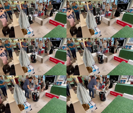
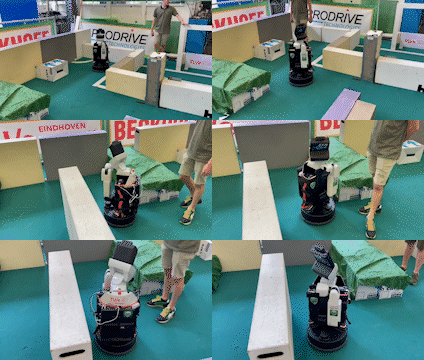
The performance during the restaurant challenge was not what the group desired. During the challenge, the robot started following its path to the first table but unfortunately hit the first corner it tried to drive around (See video on the right). The performance during testing the day before the final challenge was better than during the challenge itself (as can be seen in the video on the top). During the last test session, the robot could localize, reach the first table and avoid obstacles.
However, the performance would have looked better during the final challenge, but the code which was used for the final challenge worked a lot better on the simulation. During the last test session there were some problems with the code when the first table was reached (This also holds for the simulation). As the robot would change from global to local path planning too fast. Moreover, the global path planning was not totally correct as the starting points from the A* algorithm were sometimes not logical when the robot replanned his path. To solve this, quite some changes in code were needed and unfortunately, the changed code could only be tested on the simulation and not on the real robot before the final challenge. However, in the simulation, the code worked a lot better than previously. As the robot could perform all tasks. So it was able to localize, make a global path and avoid obstacles with local path planning. When an object was observed it could also replan its path correctly and serve all tables. This can be seen in the following video. https://tuenl-my.sharepoint.com/:v:/g/personal/j_bongers_student_tue_nl/EWhLdfZ4mLpOuJg2mS4OcfoB2HEiRW6C1aRfEXKvNvqZ5g?e=erBgD2
Nevertheless, it turned out that the parameters that worked in simulation did not do well in real life, which caused the robot to hit the first corner it encountered. During the second try of the final challenge the parameters for the local path planner were changed a bit, but unfortunately this did not have enough influence. Furthermore, the nodes could have been placed a bit further from the wall to avoid the robot driving too close to the wall. This was not really a problem in the simulation but would have been beneficial for the real robot. Despite the robot not performing as desired during the final challenge, the group knows that the robot did perform well in simulation and that it was just a matter of tweaking parameters such that the robot would perform the same in real life. FILMPJE SIMULATION
Conclusion MERLIJN
Task description
| Name | Tasks week 8 | Tasks week 9 | Tasks week 10 | Tasks week 11 |
|---|---|---|---|---|
| Lars Blommers | 1. Localisation (particle filter) | 1. Main file state flow | 1. Combine different elements in main file
2. Combine A* with localisation |
Work on wiki |
| Joris Bongers | 1. Navigation (combining global
and local navigation) |
1. Update wiki with interface,
coordinator information |
1. Combine different elements in main file
2. Combine A* with localisation |
Work on wiki |
| Erick Hoogstrate | 1. Localisation (particle filter) | 1. Finish up localisation (particle filter) | 1. Combine A* with localisation | Work on wiki |
| Noortje Hagelaars | 1. Adjust state and data diagram
after feedback from tutors 2. Navigation (A* algorithm) |
1. Robot implementation of A* | 1. Create vector map of final challenge,
node placement for A* |
Work on wiki |
| Merlijn van Duijn | 1. Navigation (A* algorithm) | 1. Robot implementation of A* | - | Work on wiki |
| Sjoerd van der Velden | 1. Adjust state and data diagram
after feedback from tutors 2. Navigation (combining global and local navigation) |
1. Update wiki with interface,
coordinator information 2. Assist with robot testing A* |
1. Combine A* with local navigation | Work on wiki |