Mobile Robot Control 2023 Group 15
Group members:
| Name | student ID |
|---|---|
| Tobias Berg | 1607359 |
| Guido Wolfs | 1439537 |
| Tim de Keijzer | 1422987 |
Practical exercises week 1:
1. On the robot-laptop open rviz. Observe the laser data. How much noise is there on the laser? What objects can be seen by the laser? Which objects cannot? How do your own legs look like to the robot.
The laser data shows with point clouds highlighted in red where objects are. In a constant environment the laser data is still quite fluid and dynamic. This indicates that there is significant noise on the robot. As of our own legs, they are visible as two small rectangles.
2. Go to your folder on the robot and pull your software.
This has been done.
3. Take your example of don't crash and test it on the robot. Does it work like in simulation?
After significant tweaking and updates, yes the simulation works.
4. Take a video of the working robot and post it on your wiki.
Video: https://youtu.be/FXOC3232ob8

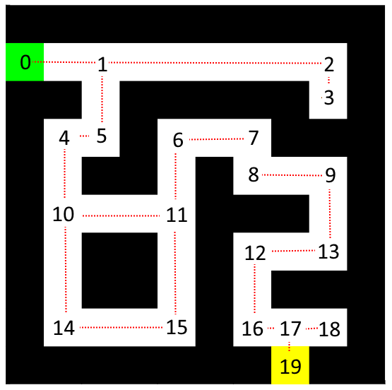
To improve the efficiency of finding the shortest path through the maze, it is suggested to decrease the number of nodes. By reducing the number of nodes, the algorithm will have to evaluate fewer nodes, which will make it more efficient.
The number of nodes can be reduced by removing nodes that are between the nodes that represent a straight line in the maze, as illustrated in Figure 1. This method results in a maze with 19 nodes, and the connections between them are indicated by red dotted lines. It is important to note that the cost of the straight paths should be updated to match the original cost of the same path. For example, the path between node 1 and 2 in the maze of Figure 1 would have a cost of 6.
The code for the Navigation-2 assignment can be found in the group repository in Gitlab, within the folder "Navigation-2".
The idea behind the used approach is based on the Artificial Potential Field Algorithm. The laser-data of the robot is used to detect objects. When these objects are within a specified range of the robot, a vector from the object to the robot is created. This vector is inversely scaled based on the distance of the object to the robot. In this approach local coordinates are used with the robot at the center of the coordinate frame. All the calculated vectors are stored in a list.
Coordinates for a goal are also defined. These are however globally defined, and are converted to local coordinates based on the odometry data of the robot. A vector from the robot to the goal is also drawn, this vector is however scaled to a fixed length, and not dependent on the distance of the robot towards the goal.
The list of vectors is summed to create a resulting force vector. Based on the orientation of this vector, the angular velocity of the robot is adjusted. The forward velocity is normally kept constant, however when the robot needs to make a very sharp turn, the robot decides to decrease the forward velocity and thus also decreasing it's turn radius.
This concept idea has resulted in the robot being able to solve the corridor maze on the simulator:
Video: https://youtu.be/9UnAluLiUOM
As well as that the robot is able to solve the corridor maze in real life during experimentation:
Video: https://youtu.be/Q__zXivK0Xg
Localization Assignment 1:
Assignment 2:

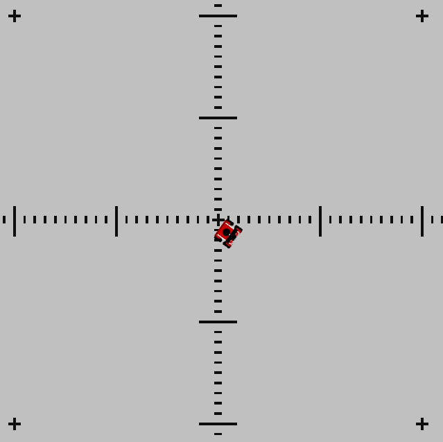
In order to determine the reliability of the odometry data in simulation, a map with distance markers was created as depicted in Figure 2. The map was used for a simulation in which the robot moved to four consecutive goals positioned on the map, forming a 5x5 meter box, and then returned to the starting point. The robot relied solely on the odometry data, employing an attractive force method derived from the artificial repulsive force code used in the navigation assignments.
In the first simulation experiment, where the uncertain_odom option was not enabled, the robot successfully reached the goals and returned to the starting point, indicating that the odometry data was dependable for navigation.
However, in the second simulation experiment with the uncertain_odom option enabled, the odometry data proved to be highly unreliable. The robot failed to reach the designated goals on the map and deviated from the starting point by more than two meters.
If the odometry data in real-life were as reliable as it was in the first simulated experiment, navigation could solely rely on this data. However, we are aware that this is not the case, and it would likely resemble the odometry data observed with the uncertain_odom option turned on. Therefore, relying exclusively on odometry data for navigation would not be a suitable approach for the final challenge.
Assignment 3: