Embedded Motion Control 2014 Group 3

Group Members

Name:	Student id:
Jan Romme	0755197
Freek Ramp	0663262
Kushagra	0873174
Roel Smallegoor	0753385
Janno Lunenburg - Tutor	-

Software architecture and used approach

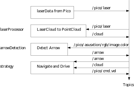
A schematic overview of the software architecture is shown in the figure below. The software basically consists only of 3 nodes, laserProcessor, arrowDetection and strategy. A short elaboration of the nodes:

laserProcessor: This node reads the /pico/laser topic which sends the laser data in polar coordinates. All this node does is converting the polar coordinates to cartesian coordinates and filters out points closer than 10 cm. Finally once the conversion and filtering is done it publishes the transformed coordinates onto topic /cloud.

arrowDetection: This node reads the camera image from topic /pico/asusxtion/rgb/image_color and detects red arrows. If it detects an arrow the direction is determined and posted onto topic /arrow.

strategy: This node does multiple things. First it detects openings where it assigns a target to, if no openings are found the robot finds itself in a dead end. Secondly it reads the topic /arrow and if an arrow is present it overrides the preferred direction. Finally the robot determines the direction of the velocity of the robot using the Potential Field Method (PFM) and sends the velocity to the topic /pico/cmd_vel.

The approach is very simple and easy to implement. The strategy node for example has approximately only 100 lines of code. The benefit of easy code is the easiness to tackle bugs and that bugs are less likely to occur. Another benefit of this 'simple' code is the easiness to optimize for performance.

Applied methods description

Arrow detection

The following steps describe the algorithm to find the arrow and determine the direction:

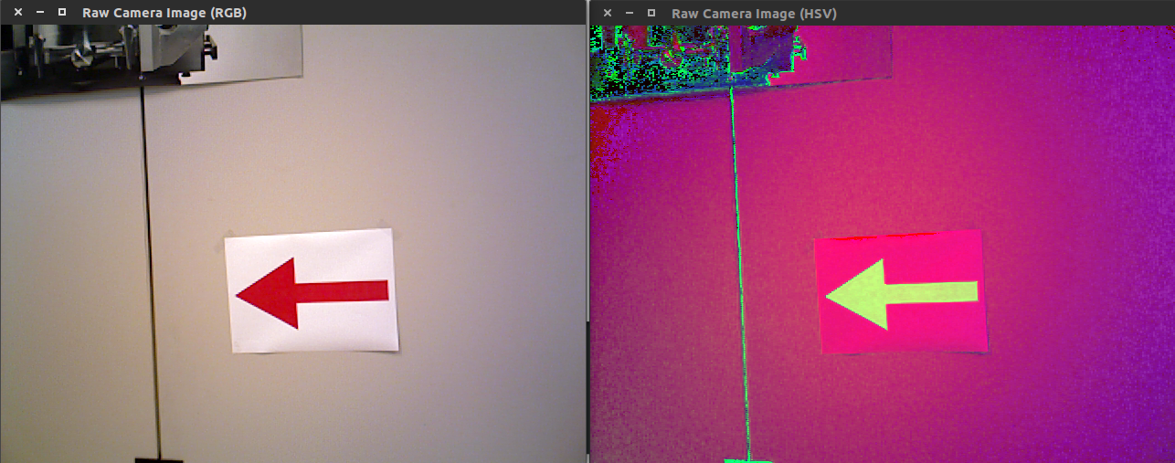
1. Read rgb image from "/pico/asusxtion/rgb/image_color" topic.

2. Convert rgb image to hsv color space.

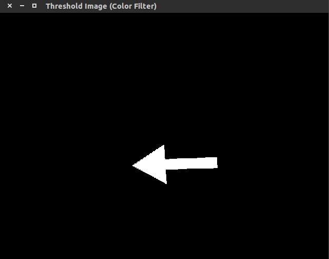
3. Filter out the red color using cv::inRange

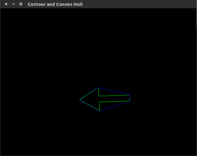
4. Find contours and convex hulls and filter it

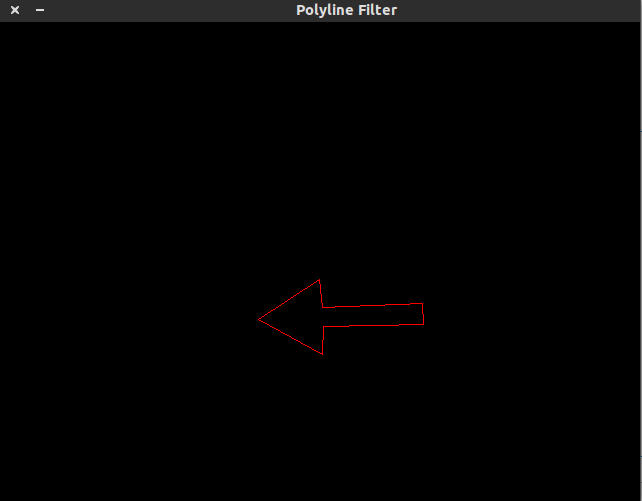
The filter removes all contours where the following relationship does not hold: [math]\displaystyle{ 0.5 \lt \frac{Contour \ area}{Convex \ hull \ area} \lt 0.65 }[/math]. This removes some of the unwanted contours. The contour and convex hull of the arrow:

5. Use cv::approxPolyDP over the contours

The function cv::approxPolyDP is used to fit polylines over the resulting contours. The arrow should have approximately 7 lines per polyline. The polylines fitted over the contours with [math]\displaystyle{ 5 \ \lt \ number \ of \ lines \ in \ polyline \ \lt \ 10 }[/math] is the arrow candidate.

6. Determine if arrow is pointing left or right

First the midpoint of the arrow is found using [math]\displaystyle{ x_{mid} = \frac{x_{min}+x_{max}}{2} }[/math]. When the midpoint is known the program iterates over all points of the arrow contour. Two counters are made which count the number of points left and right of [math]\displaystyle{ x_{mid} }[/math]. If the left counter is greater than the right counter the arrow is pointing to the left, otherwise the arrow is pointing to the right.

7. Making the detection more robust As last an effort is made to make the arrow detection more robust, for example when at one frame the arrow is not detected the program still knows there is an arrow. This is done by taking the last 5 iterations, check if in all these iterations the arrow is detected then publish the direction of the arrow onto the topic "/arrow". If in the last 5 iterations no arrow is seen the arrow is not visible anymore thus publish that there is no arrow onto the topic "/arrow".

Strategy

Target

In the approach used a targed is needed for Pico to drive to. In this section the determination of the target point is explained. In the code a loop is made through all data points, which are in order from right to left. Only the points within 1.4 meter from pico are encountered. If the distance between two following points is bigger than a determined threshold, the presence of a door is assumed. This will be further explained with the following figure.

In the figure the vision of pico is illustrated by the dotted black arc and the detected points within this marge by red dots. In the left figure two distances between following points are bigger than the given threshold and thus two doors are present. The targets are set in the middle of the line between the two points. In the figure in the middle a problem is illustrated which occured during testing. When Pico looks past a corner it sometimes sees points where no walls are, the so called ghostpoints. This is a problem because in the case of ghostpoints the distance between two points becomes smaller than the threshold. To filter this effect the distance is not taken between two points, but over five. By testing and tuning the value of five was found as an optimal. A downside of this method is that points far ahead of pico give the possibility of false positives. But because in this case Pico only looks at a relative short distance, this will not occur.

First software approach

Obstacle Detection

Finding Walls from PointCloud data

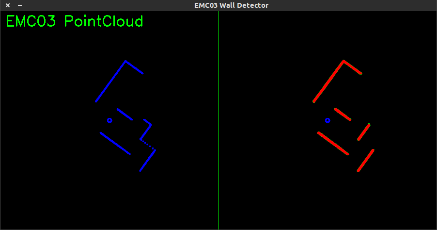
The node findWalls reads topic "/cloud" which contains laserdata in x-y coordinates relative to the robot. The node findWalls returns a list containing(xstart,ystart) and (xend, yend) of each found wall (relative to the robot). The following algorithm is made:

- Create a cv::Mat object and draw cv::circle on the cv::Mat structure corresponding to the x and y coordinates of the laserspots.

- Apply Probabilistic Hough Line Transform cv::HoughLinesP

In the picture shown below one can see the laserspots at the left side of the picture. At the right side the lines of the cv::HoughLinesP are shown.

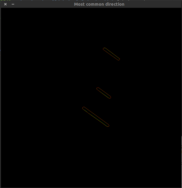
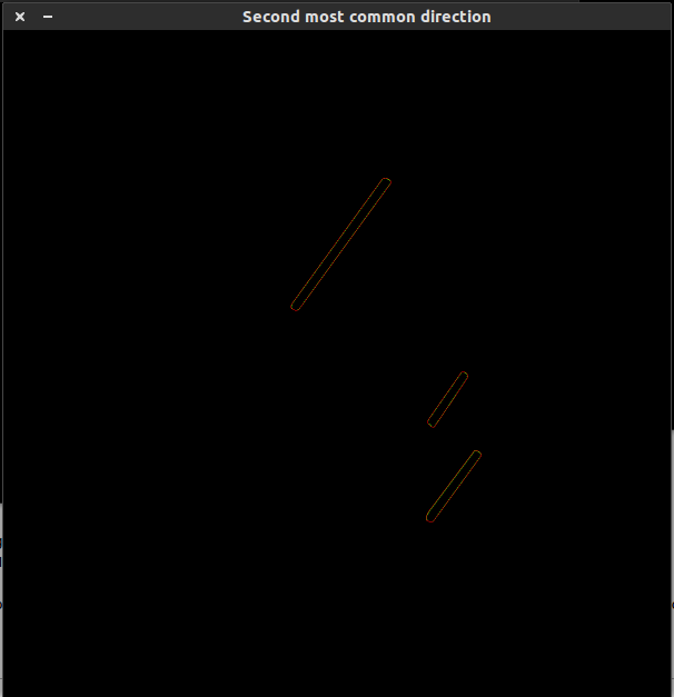
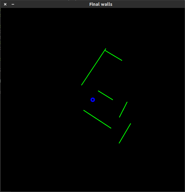
The cv::HoughLinesP algorithm gives multiple lines per wall. In the end we want 1 line per wall. To solve this first the all the lines are sorted into lists by their angle they make, for example if a line makes angle of [math]\displaystyle{ 27^\circ }[/math] it is stored in a list where all lines lie between [math]\displaystyle{ 20^\circ }[/math] and [math]\displaystyle{ 30^\circ }[/math]. Once all lines have been sorted the two most common directions are plotted which is shown in the following pictures:

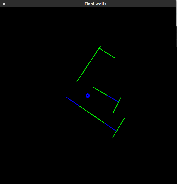
Finally to extract 1 line per wall the outer points of the contour are taken to get 1 line per wall. The result is shown in the following figure:

Finding Doors from found Walls

Now that the walls are given as lines doors are fitted between the walls. The result is shown in the following figure:

Why this method doesn't work in real life

The method described in how to find walls and doors did not work properly in real life. We experienced some serious robustness problems due to the fact that in some of the iterations complete walls and/or doors were not detected, thus the robot couldn't steer in a proper fashion to the target. Secondly this method required some serious computation power which is not preferable (one cpu core ran at 80% cpu when the refresh rate of the algorithm was only 5 Hz).