Embedded Motion Control 2019 Group 2
Group members
| Name | Student number |
|---|---|
| Bob Clephas | 1271431 |
| Tom van de laar | 1265938 |
| Job Meijer | 1268155 |
| Marcel van Wensveen | 1253085 |
| Anish Kumar Govada | 1348701 |
Introduction
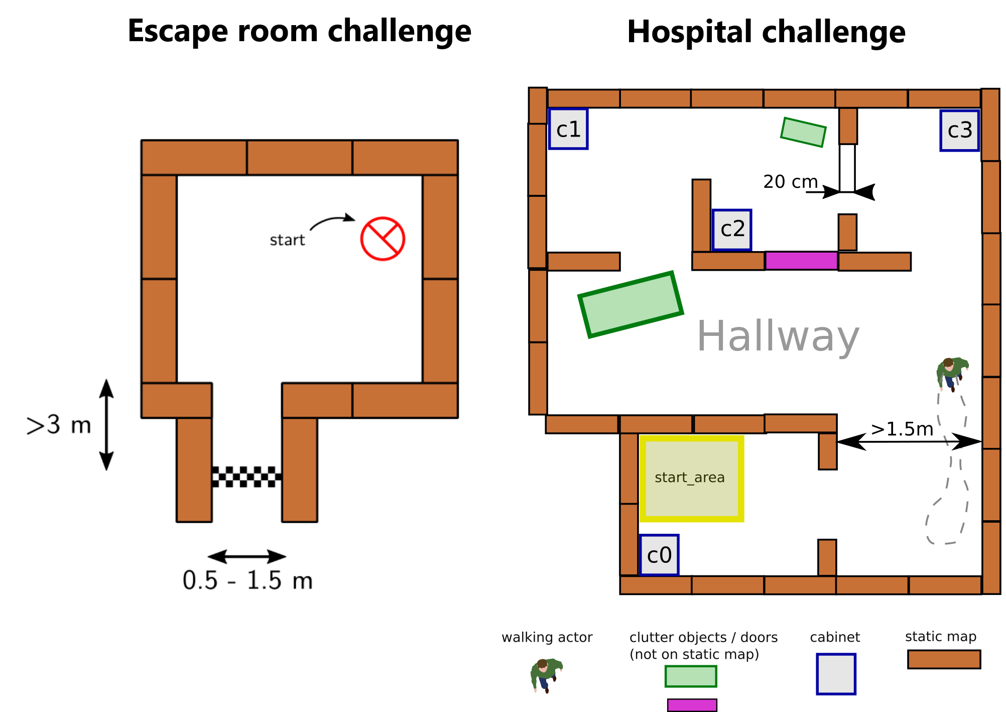
Welkom on the wiki of group 2 of the 2019 Embedded motion control course. During this course the group has design and implemented their own software which allows a PICO robot to complete two different challenges autonomously. The first challenge is the "Escape room challenge" where the PICO robot must drive out of the room from a given initial position inside the room. In the second challenge called the "Hospital challenge" the goal is to visit an unknown number of cabinets in a specified order, placed in different rooms. For both challenges the group designed one generic software structure that is capable of completing both challenges without changing the complete structure of the program. In figure 1 the maps of both challenges are shown to give a general idea about the challenges. On the general wiki page of the Embedded motion control course 2019 (link) the full details are given regarding both challenges.
Design document
To complete the two assignments for the course “Embedded motion control” specific software must be written. In this design document the global architecture of the software is explained, and the given constraints and hardware is listed. This document is created and used at the first weeks of the course and can be found here.
The most important points from the design document are shown below:
Requirements and specifications
| Requirements | Specifications |
|---|---|
| Accomplish predefined high-level tasks | 1. Find the exit (Escape room challenge)
2. Reach a predefined cabinet (Hospital Competition) |
| Knowledge of the environment | 1. Location of walls (via corner points)
2. Location of the doors (via corner points) 3. Location of the cabinets (via corner points) 4. Location of static objects (via corner points) 5. Location of dynamic objects (via corner points) 6. Map at 2D level 7. Accuracy of 0.1 meter |
| Knowing where the robot is in the environment | 1. Know the location at 2D level
2. XY with < 0.1 meter accuracy 3. Orientation (alpha) with <10 degree accuracy |
| Being able to move | 1. Max. 0.5 [m/s] translational speed
2. Max 1.2 [rad/sec] rotational speed 3. Able to reach the desired position with <0.1 meter accuracy 4. Able to reach the desired orientation with <0.1 radians accuracy |
| Avoid obstacles | 1. Never bump into an object
2. Being able to drive around an object when it is partially blocking the desired path |
| Standing still | 1. Never stand still for longer than 30 seconds |
| Finish as fast as possible | 1. Within 5 minutes (Escape room challenge)
2. Within 10 minutes (Hospital Competition) |
| Coding language | 1. Only allowed to write code in C++ coding language
2. GIT version control must be used |
Software components
| Software block | Specifications |
|---|---|
| World model | 1. Storing all the relevant data (Map / tasks / position/ etc.)
2. Data communication between the other components (All data goes through the world model) |
| Task manager | 1. Set operation modes of other blocks depending on the current status of the blocks and high level tasks |
| Perceptor | 1. Reading sensor data
2. Identifying walls and objects based on laser data and create local map 3. Fit local map onto global map (Hospital Competition) 4. Locate robot on local map (Escape room challenge) 5. Locate robot on global map (Hospital Competition) 6. Keep local map aligned with global map (Hospital Competition) |
| Path planner | 1. Create a path from the combined map, current position and the desired position
2. Check if path is free and plan new path if current path is blocked 3. Keep track of open and closed doors |
| Drive controller | 1. Actuates the robot such that it arrives at the desired location (keep speed and acceleration in mind)
2. Check if the desired direction is safe to drive to (based on laser data obtained from perceptor, not based on the map) |
Hardware components
| Software block | Specifications |
|---|---|
| PICO Robotic platform | Jazz telepresence robot |
| Sensors | Laser range finder - Scan environment and detect objects
Wheel encoders - Determine the traveled distance by the wheels |
| Actuators | Holonomic base (omni-wheels) - Allows the robot to move on the ground |
| Computer | Intel I7 processor
OS: Ubuntu 16.04 (64-Bit) ROS with own software layer |
Environment
| Challenge | Specifications |
|---|---|
| Escape room challenge | 1. Rectangular room, unknown dimensions. One opening with a corridor.
2. Starting point and orientation is random, but equal for all groups. 3. Opening will be perpendicular to the room. 4. Far end of the corridor will be open. 5. Wall will not be perfectly straight, walls of the corridor will not be perfectly parallel. 6. Finish line is at least 3 meters in the corridor, walls of the corridor will be a little bit longer. |
| Final Challenge | 1. Walls will be approx. perpendicular to each other
2. Global map is provided before competition 3. Location of cabinets is provided in global map 4. Static elements, not showed in global map, will be in the area 5. Dynamic (moving) elements will be in the area 6. Objects can have a random orientation 7. Multiple rooms with doors 8. Doors can be open or closed 9. list of "To-be-visited" cabinets is provided just before competition |
General software architecture and interface
The overall software is split into several building blocks such as the Task manager, World model, Perceptor, Path planner, Drive controller and the respective data flow between them as shown in the figure below :
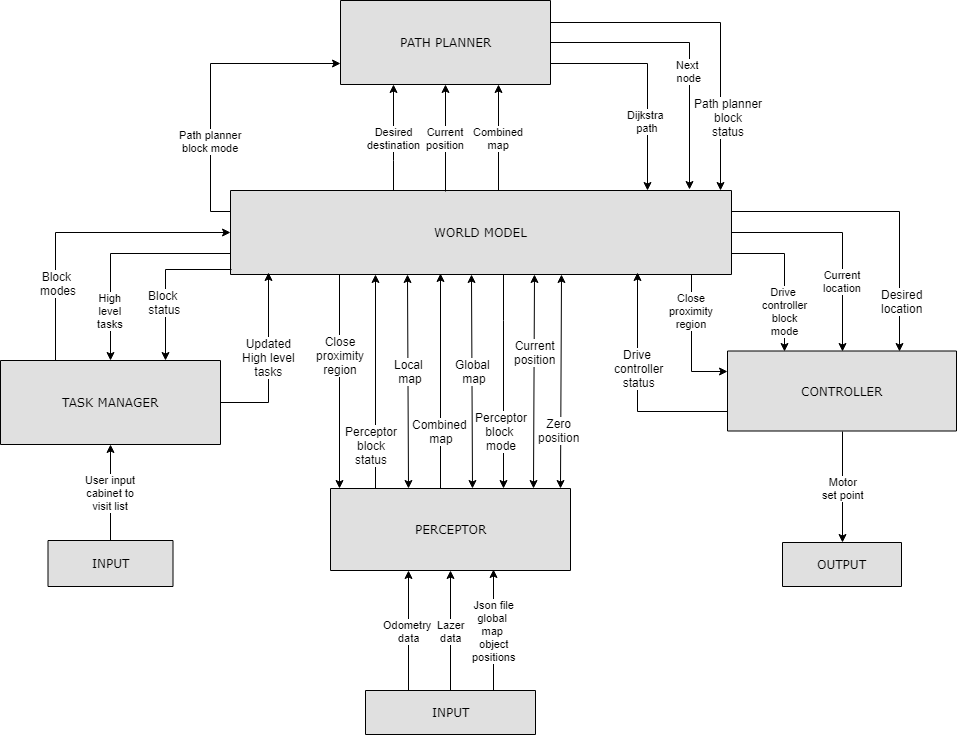
Data flow
| Block | Data | Transition from | Transition to | Block | Data | Transition from | Transition to |
| Perceptor | Lazer range finder data | LRF Sensor input | Perceptor | Path planner | Desired destination | World model | Path planner |
| Odometry data | ODO Sensor input | Perceptor | Current position | World model | Path planner | ||
| Json file - Global Map and location of cabinets | File read | Perceptor | Combined map | World model | Path planner | ||
| Perceptor block modes | World model | Perceptor | Path planner block mode | World model | Path planner | ||
| Local map | World model | Perceptor | Path planner block status | Path planner | World model | ||
| Global map | World model | Perceptor | Next node | Path planner | World model | ||
| Current position | World model | Perceptor | Path from Dijkstra algorithm | Path planner | World model | ||
| Zero position | World model | Perceptor | Drive controller | Desired location/Next node | World model | Drive controller | |
| Global map | Perceptor | World model | Current location | World model | Drive controller | ||
| Perceptor block status | Perceptor | World model | Close proximity region | World model | Drive controller | ||
| Local map | Perceptor | World model | Drive controller block mode | World model | Drive controller | ||
| Combined map | Perceptor | World model | Drive controller block status | Drive controller | World model | ||
| Zero position | Perceptor | World model | Motor set point | Drive controller | Output | ||
| Current position | Perceptor | World model | |||||
| Close proximity region | Perceptor | World model | |||||
| Task manager | User input cabinet list | User | Task manager | ||||
| Block status | World model | Task manager | |||||
| High level tasks | World model | Task manager | |||||
| Block modes | Task manager | World model | |||||
| Updated high level tasks | Task manager | World model |
Overall program flow
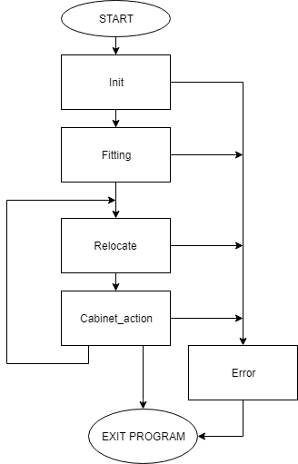
The overall program is divided in 5 phases. During a phase all actions lead to one specific goal. When the goal is reached, a transition is made towards a new phase. Within a phase it is possible to have multiple cases. Each iteration of the program it is evaluated to what phase and case the program should move. It is also possible to stay in a specific phase and case for longer than one program iteration, however, in most situations this is not needed. Every case has a specific block mode for each software block and the transitions between cases and phases is based on the blockstatusses of all blocks.
Phases flowchart
In figure 2 the overall structure with the phases is shown. The different phases have the following goals:
Init phase
The init phase focuses on the initialisation of the program. This phase has one case and the flowchart of this phase is shown in figure 3.
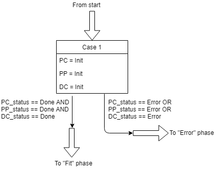
During the init phase the following actions are executed:
Fitting phase
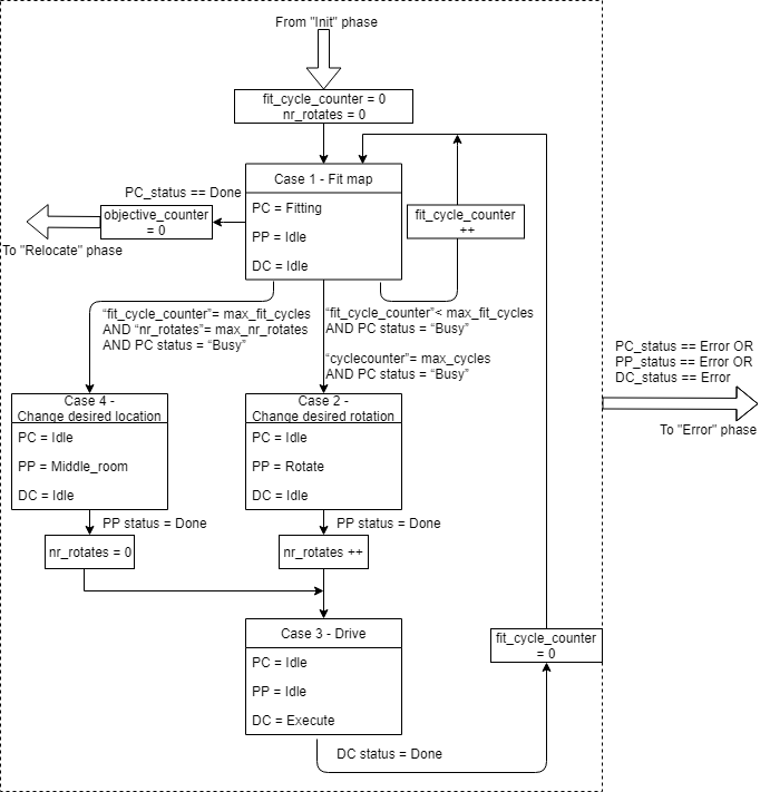
In the fitting phase the goal is to locate the robot relative to the given global map. This fitting is done in the perceptor by checking the laserdata, creating a local map and try to find a best fit between the local and global map. If this fit is successful the location of the robot is known and all new laser information can be used to update the location of the robot.
Relocate phase
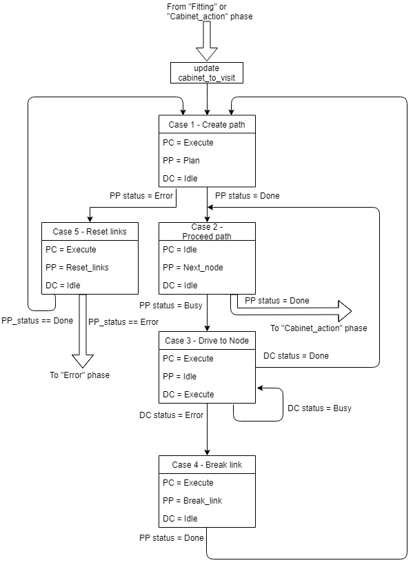
In the "Relocate" phase the goal is to drive the robot to the next cabinet. The driving involves the path planning, actuating the drivetrain of the robot and avoiding obstacles. During the driving the perceptor keeps updating the world map and keeps adding objects to the map is necessary. Also the fitting will be improved once more laserdata is obtained.
In figure 5 the overall flowchart is shown of the relocate phase. This phase contains the following cases:
Cabinet_action phase

During the cabinet action phase the robot can interact with the cabinet.
The required interaction is specified in the competition and is consisting of taking a snapshot of the current laserdata and play a sound.
The flowchart of this phase is shown in figure 6.
Error phase
The error phase is only visited if something unrecoverably went wrong in the program, e.g. a required file is missing. In this phase the output of the drive motors is set to zero and the error is displayed to the user. Then the program is terminated
Software blocks
World model
The world model is the block which stores all the data that needs to be transferred between the different blocks. It acts as a medium of communication between the various blocks such as perception, task manager, path planner and drive controller. It contains all the get and set functions of the various blocks to perform respective tasks.
As seen in the data flow table, the various input data and output data that are sent in and out of the world model are accessed using get and set functions.
Input
- Updated high level tasks - Task manager
- Block modes - Task manager
- Block statuses - All blocks
- Close proximity region - Perceptor
- Current position - Perceptor
- Zero position - Perceptor
- Global map - Perceptor
- Local map - Perceptor
- Combined map - Perceptor
- Next node - Path planner
- Path from Dijkstra algorithm - Path planner
Output
- High level tasks - Task manager
- Block statuses - Task manager
- Block modes - Drive controller, Perceptor and Path planner
- Close proximity region - Drive controller
- Current location - Drive controller, Path planner
- Desired location/ next node - Drive controller
- Current position - Perceptor
- Zero position - Perceptor
- Global map - Perceptor
- Local map - Perceptor
- Combined map - Path Planner
- Desired destination/ next cabinet node - Path planner
Task manager
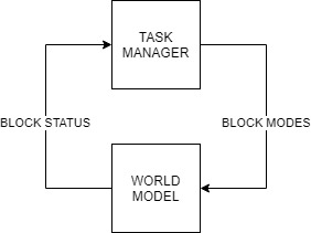
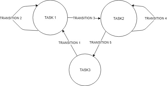
The task manager functions as a finite state machine which switches between different tasks/states. It focuses mainly on the behavior of the whole program rather than the execution. It determines the next operation phase and case based on the current phase, current case, current block statuses and counters in which the corresponding block modes of the perceptor, path planner and drive controller are set for the upcoming execution. It communicates with the other blocks via the World model.
Since the "Escape room challenge" and the "Hospital competition" require a complete different approach in terms of cooperation between the blocks, the task planner is completely rewritten for both challenges.
ESCAPE ROOM CHALLENGE
BASIC BLOCK DIAGRAM :
INITIALIZATION:
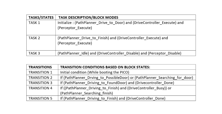
The path planner is given a command “Drive_to_door” while the drive controller and the preceptor are given a command “Execute” as a part of the initialization process.
EXECUTION:
The high-level tasks “Drive_to_door”, “Drive_to_exit”, “Execute”, “Idle” and “Disable” were given to appropriate blocks as shown below:
KEY:
HOSPITAL ROOM CHALLENGE
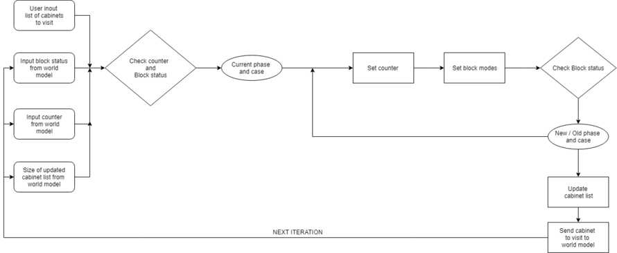
The task manager is completely revamped for the hospital challenge. It functions as a state machine and handles the behavior of the program in a well structured manner considering various fall back scenarios which can be edited when ever needed. The list of cabinets to visit are initially read by the task manager and sent to the world model. . It works primarily on setting appropriate block modes, setting counter variables and changing from a particular phase and case of the program to another in order to perform a required task based on the block statuses it receives. The various phases and cases are discussed further in the Overall Program flow section. The functions of the task manager are described in the flowchart below :
FLOW CHART :
The function description can be found here : File:TASK MANAGERfin.pdf
Perceptor
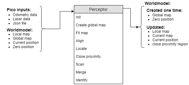
The perceptor receives all of the incoming data from the pico robot and converts the data to useful data for the worldmodel. The incoming data exists of odometry data obtained by the wheel encoders of the pico robot. The laserdata obtained by the laser scanners. A Json file containing the global map and location of the cabinets, this file is provided a week before the hospital challenge. Moreover, the output of the perceptor to the world model consists of the global map, a local map, a current map, the current/zero position and a close proximity region. The incoming data is handled within the perceptor by the following functions. A detailed description on what each function does in the preceptor and more information about the data flow can be found here.
The inputs and outputs of the perceptor are shown in the following figure:
Init position
The pico robot saves the absolute driven distance since its startup. Therefore, when the software starts it needs to reinitialize the current position of the robot. If the robot receives its first odometry dataset it saves this position and sets it as zero position for the worldmodel. This happens only once when the software is started.
create global map
Close proximity
Dynamic objects are not measured by the local map. To prevent collisions with the robot and a dynamic objects or walls, a close proximity region is determined. This region is described as a circle with the configured radius around the robot. The function returns a vector describing the measured distances of a filtered set of laser range finder data points to the worldmodel.
Locate
This function makes use of the zero-frame which is determined by the init function. Once the odometry data is read a transformation is used to determine the position of the robot with respect to the initialized position. This current position is outputted to the worldmodel.
Fit map
For the pico robot to know where it is located on the given global map, a fit function is created.
Align
Scan
The laserdata is read from the sensor, however, this data is in polar coordinates. Therefore, the data is first transformed to Cartesian coordinates. Next, the data is resampled so there is a minimum set distance between all of the data points. This resampled data is used to calculate the angles between all the consecutive points. To determine which data points represent a wall the data is split in different clusters. The data is splitted using an average angle of the cluster and the angle of the next point. Therefore, the data is split at the corners of each wall. Lastly, the points of each cluster are marked as a wall with floating points at both sides of the walls also the position of these floating points is stored as well. This stored information of the end points of walls is defined as current map.
Merge
In this function the new laser data is merged with an existing map to form a more robust and complete map of the environment. Therefore, laser data in the form of a current map created by the scan function is imported. Furthermore, the previous created output of the merge function is imported as well, which is called the local map. Firstly, the previous created map is transformed to the current position of the robot. Secondly, similar walls are merged. Walls are considered to be similar if they are parallel to each other, have a small difference in angle or are split into two pieces. If two walls are close to each other but one has a smaller length they are merged as well. The merge settings are stored in the configuration file. The different merge cases can be seen in figure … . Once similar walls are merged, the endpoints of walls are connected to form the corners points of the room. Each point of a wall has a given radius, and if another point has a distance to this point which is smaller than its radius then the points will be connected. To improve the robustness of the local map the location of these corner points is mainly based on the location of the corner points from the previous local map, which ensures rejection of measurement errors in the laser data. Furthermore, the wall points that are not merged or connected at the end of the function will be removed. Therefore, the local map will only consist of walls which are connected to each other.
Identify
The functionality of this function is to identify the property of the points in the local map. For instance corner points can be convex or concave. This property is later used to help identify doors, objects or cabinets in the local map. The position of the robot determines if the corner point is convex or concave. With this property information the map is scanned for doors. For the escape room challenge a door is identified as two convex points close to each other. A door is defined between two walls, these walls should be approximately in one line. Also, the corner points cannot be from the same wall to further increase the robustness of the map. It is unlikely that the local map immediately contains two convex points which can form a door. Therefore, a possible door is defined, so the robot can drive to the location and check if there is a real door at this position. There are multiple scenarios where a possible door can be formed. Such as, one convex point and one loose end, two loose ends or a loose end facing a wall. Concave points can never form a door and are therefore excluded. When forming a possible door the length of the door and the orientation of the walls is important as well.
Path planner
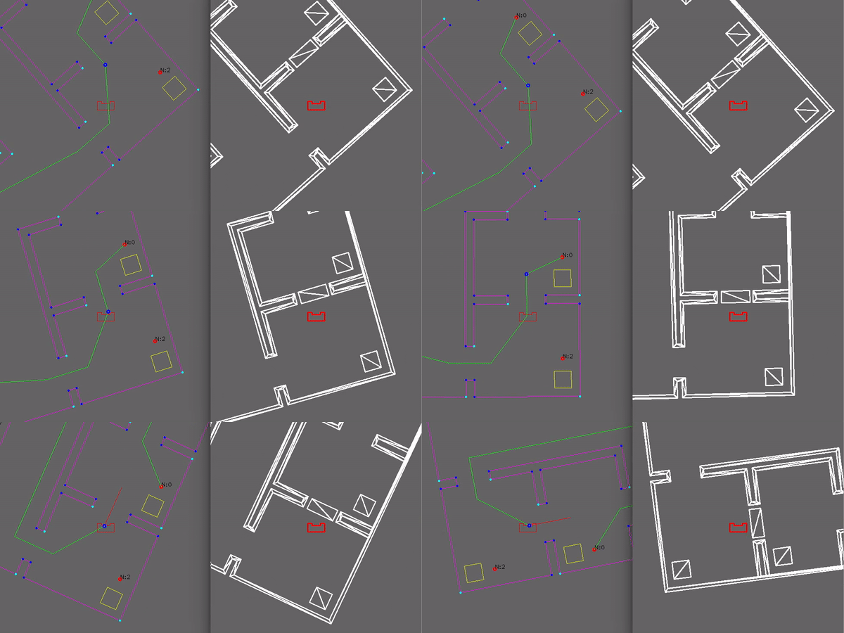
For planning paths the choice is made to use nodes that are placed at the following locations:
- In front of a door (one at each sides)
- In front of a cabinet
- In the starting area
- Distributed over each room in order to plan around objects, eg. in the middle
Gridding the map is also considered but was not chosen because of the higher complexity and with separate nodes debugging is easier as well. The path planner determines the path for the PICO robot based on the list of available nodes and the links between these nodes. For planning the optimal path, Dijkstra's algorithm is used and the distance between the nodes is used as a cost. The choice for Dijkstra is based on the need for an algorithm that can plan the shortest routhe from one node to another. Also it was selected on being sufficient for this application, the extra complexity of the A* algorithm was not needed. The planned path is a set of positions that the PICO robot is going to drive towards, this set is called the ‘next set of positions’. This next set of positions is saved in the world model and used by the task manager to send destination points to the drive controller. In figure 7 is shown how the path planner behaves in case of a closed door: the link is broken and a new path around the closed door is planned.
The path planner takes the desired destination, current position, list of all available nodes and the path planner block mode as inputs. The functions of the path planner are idling, planning a path, setting the next node of the planned path as current destination position, breaking a link between nodes, resetting all broken links and rotating the PICO robot. This results in the planned path (next set of positions), the destination position and the path planner block status. The inputs, functions and outputs of the path planner are visualized in the following figure:

All functions of the path planner are explained below.
Idle
When idling, all variables are set to their initial value and the path planner waits for the task manager to set the block mode. When the path planner is idling, the block status changes to idling.
Plan paths
In this function all possible paths to the desired destination are planned based on the combined map. The combined map contains a list of doors, which contain two ‘nodes’ each. A node is a location point in front of the door, and since the door has two sides there are two nodes for each door. Also is checked if there are no objects, for example a wall or cabinet, in between these nodes. The planned path consists of a <Position> vector, where only the positions are listed where the PICO robot has to stop and rotate. All possible planned paths, for example through different doors, are stored in one vector and the optimal path is selected later.
Set next node
Once all possible paths are planned, PICO has to follow it. To do this, the list of nodes from the created path is followed. The next node is set if the task manager changes the mode of the path planner to set next node.
Break link
If PICO is not able to reach a node, the link between the current destination node and the last node must be broken. This is done when the task manager sets the block mode to break link.
Reset broken links
When there is no possible path because all links are broken, the broken links are set to open again and a path is planned. This is implemented in case a dynamic obstacle was blocking the path. This function is called when the task manager changes the block mode to reset broken links or when the plan path function cannot create a path towards the given destination.
Rotate
When PICO has to scan the room, it must be able to rotate. Using the rotate function the desired destination of PICO is changed, where the angle is adjusted by the in this function inserted value.
A detailed description of the path planner can be found here.
Drive controller
The drive controller software block ensures that the pico robot drives to the desired location. it receives the current and desired location and automatically determines the shortest path towards the desired location. While driving it also avoids small obstacles on it's path. If the object is too large, or the path is blocked by a door for example, the drive controller signals this to the path planner which calculated an alternative path.
To avoid obstacles a potential field algorithm is implemented in the drive controller. This algorithm uses two types of forces which are added and used to find a free direction. The first force is an attractive force towards the desired location. Secondly all the objects (walls, static and dynamic objects) that are close to the robot have a repellent force away from them. The closer the object, the larger the repellent force. All the forces are added together and the resulting direction vector is determined. This new direction is used as a desired direction at that time instance. In the gif shown here the repellent forces are visualised and it can be seen that Pico uses this to drive around an object in its path. The green points are showing the free directions and in red the directions towards an object, together with an arrow visualising the repellent force.
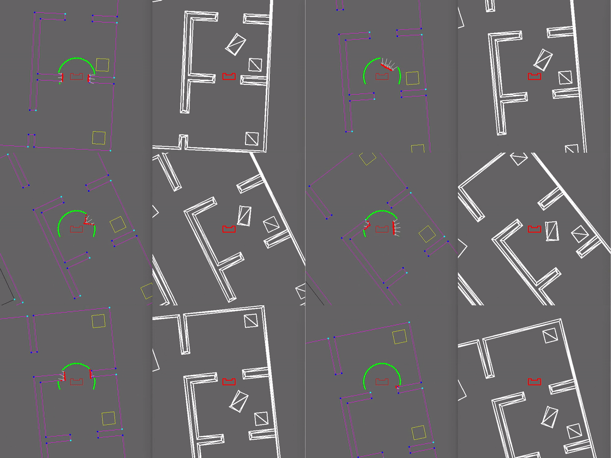
More details of the Drive Controller, including function descriptions can be found in the Drive Controller functionality description document found here.
Visualisation
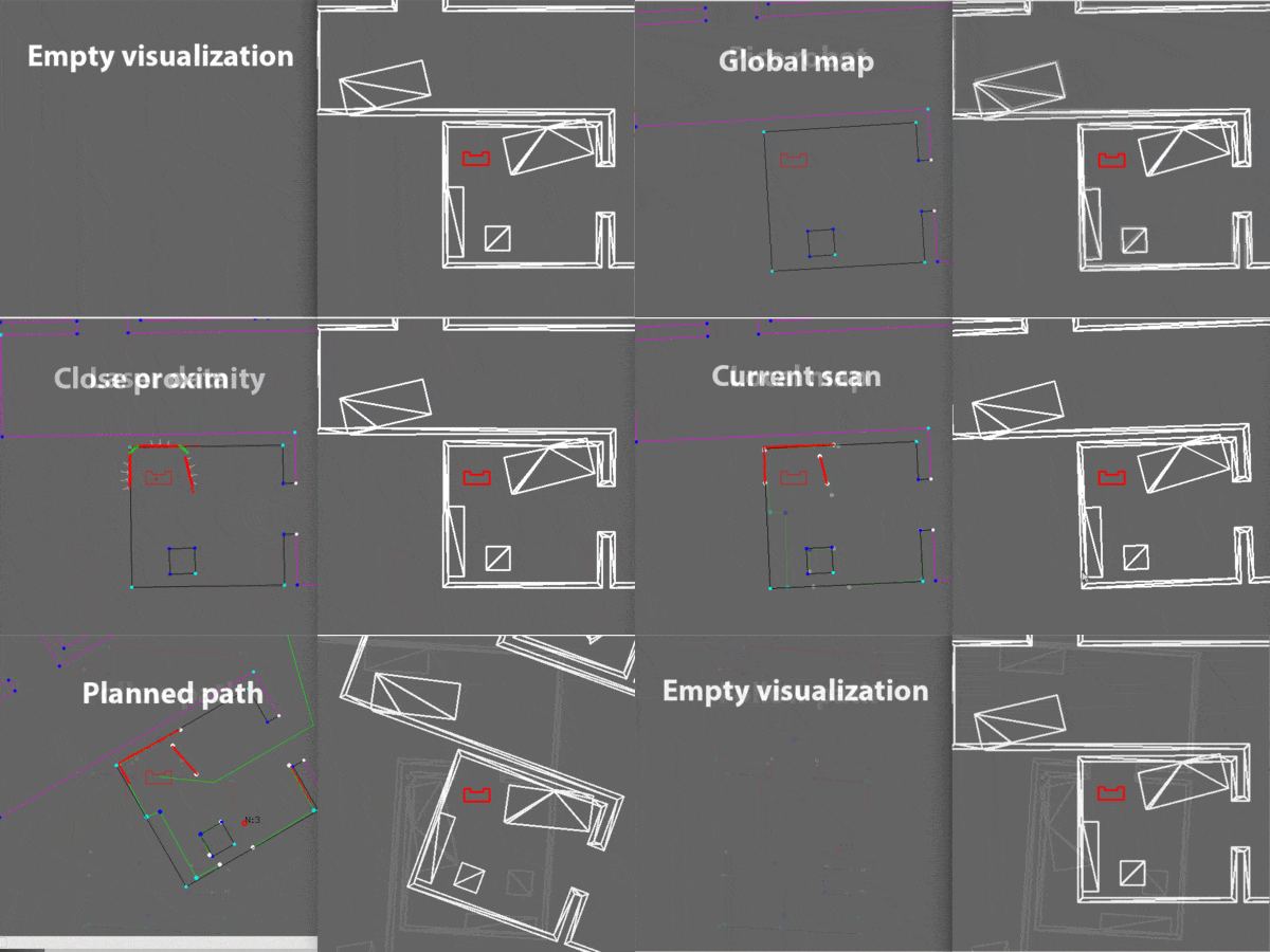
To make the debugging of the program faster and more effective a new class in the software is added. This visualization class draws an empty canvas of a given size. With one line of code the defined objects can be added to this canvas. Each loop iteration the canvas is cleared and can be filled again with the updated or new objects. The visualization class is excluded from the software architecture. There is chosen to not include this class in the software architecture, because, class has no real functionality except for debugging. Any other software block can make use of the visualization to quickly start debugging. However, the visualization is especially used in the main to prevent unclarities. All objects that are visualized in the main have to exist in the world model.
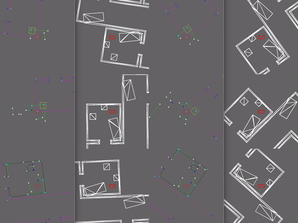
The visualization makes use of the opencv library and a few of its basic functionalities such as imshow, newcanvas, Point2d, circle, line and putText. The struct "object" that can be added to the visualization is as defined in the code snippet "class definition". The struct can contain a object type, points, connection between points, point properties and visualization color. For example, in the visualization can be seen if points are connected (blue) or not (white). Moreover, darker blue points indicate that the corner is concave, light blue points indicate convex corners with respect to the robot. The maps as defined in the world model can also be visualized. Those maps are created using a vector of objects. In figure ... example objects are visualized. A few examples that are visualized, The laser range finder data, those are visualized as red dots. The close proximity region is visualized using red and green dots. In this case a green dot indicates a direction contains no objects, a red dot indicates an object is within the defined region. Furthermore, arrows are used to visualize how close the object is to the robot. This region is used by the drive controller for the potential field algorithm. TODO Current scan, local map , global map, planned path. nodes.
Challenges
Escape Room Challenge
Our strategy for the escape room challenge was to use the software structure for the hospital challenge as much as possible. Therefore, the room is scanned from its initial position. From this location a local map of the room is created by the perceptor. Including, convex or concave corner points, doors and possible doors (if it is not fully certain the door is real). Based on this local map the task manager gives commands to the drive controller and path planner to position in front of the door. Once in front of the the possible door and verified as a real door the path planner sends the next position to the world model. Which is the end of the finish line in this case, which is detected by two lose ends of the walls. Also the robot is able to detect if there are objects in front of the robot to eventually avoid them.
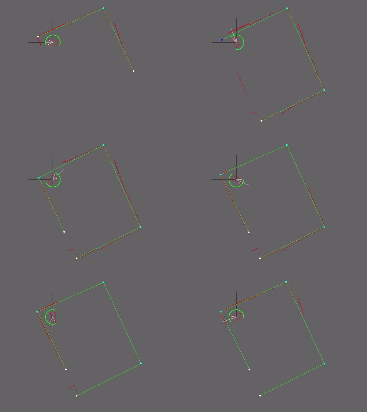
Simulation and testing
Multiple possible maps where created and tested. In most of the cases the robot was able to escape the room. However, in some cases such as the room in the escape room challenge the robot could not escape. The cases were analyzed but there was enough time to implement these cases. Furthermore, the software was only partly tested with the real environment at the time of the escape room challenge. Each separate function worked, such as driving to destinations, making a local map with walls, doors and corner points, driving trough a hallway and avoiding obstacles.
What went good during the escape room challenge:
The robot was made robust, it could detect the walls even though a few walls were placed under a small angle and not straight next to each other. Furthermore, the graphical feedback in from of a local map was implemented on the “face” of the Pico. The Pico even drove to a possible door when later realizing this was not a door.
Improvements for the escape room challenge:
Doors can only be detected if it consists of convex corners, or two loose ends facing each other. In the challenge it was therefore not able to detect a possible door. The loose ends were not facing each other as can be seen in the gif below. Furthermore, there was not back up strategy when no doors where found, other then scanning the map again. Pico should have re-positioned itself somewhere else in the room or the pico could have followed a wall. However, we are not intending to use a wall follower in the hospital challenge. Therefore, this does not correspond with our chosen strategy. Another point that can be improved is creating the walls. For now walls can only be detected with a minimal number of laser points. Therefore, in the challenge it was not able to detect the small wall next to the corridor straight away. This was done to create a robust map but therefore also excluded some essential parts of the map.
In the simulation environment the map is recreated including the roughly placed walls. As expected in this simulation of the escape room the pico did not succeed to find the exit, the reasons are explained above.
Hospital Challenge
During the hospital challenge a list of cabinets in a hospital must be visited to pick and place medicine. The given order of cabinets was 0, 1 and finally 3. Before this challenge a global map of the hospital with coordinates of the cabinets and walls was given. However there are doors that might be closed and unknown objects in the hospital. These objects can be either static or dynamic. The PICO robot must be able to handle these uncertainties.
The software for the hospital challenge is an improved version of the software used during the escape room challenge. The same block structure is used and as much as possible software is reused and adjusted where necessary. Major changes are done to the path planner and task manager since the complexity of the hospital challenge is much higher for those two blocks compared to the escape room challenge.
Video
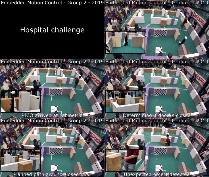
The full and higher quality version of the video can be found here: Hospital challenge - video group 2 - 2019
What went well
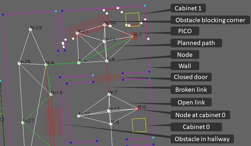
The things that went well where being able to detect various objects such as walls and doors correctly. Next to that the closed door and static object were detected properly. Furthermore being able to plan a path around the closed door and static obstacles was no problem. Planning around objects is done by breaking the links between nodes, such that the path planning algorithm does not use these broken links anymore while planning a path. The broken links during the hospital challenge are visible in Figure 8 where all red lines between nodes indicate a broken link, white lines indicate a open link and the green lines indicate the planned path. Also did the localization work well, once it had determined the starting position correctly. This made it possible to determine the correct position of the PICO robot in the hospital during the challenge. Also was the localization robust against disturbances that were blocking it from detecting corners of rooms. This is also visible in Figure 8, where an object was blocking the top left corner of the room where PICO was in at that moment while visiting cabinet 1.
Improvements for the hospital challenge
The things that we would improve are improving the initial localization robustness since during the first try the localization was off, resulting in PICO getting stuck in the hallway. Luckily it did work correctly after a restart and we were able to finish. Also did we slightly hit the obstacle in the hallway, which was unexpected since a protection mechanism to avoid running into objects is implemented. Why this happened has to be investigated. The last improvement is reducing the total time to finish the challenge. The driving speed was lowered during the challenge to improve the accuracy of the localization, because the detected walls and doors were slightly off. If the robustness of the localization is improved, the driving speed can be increased as well to finish the hospital challenge faster. The time duration can also be decreased by removing the delay while waiting at a cabinet, since this delay was set to 5 seconds.
Code snippets
Looking back at the project
What went good
When looking back at the project, several things went well. Firstly, a good structure was set up before we started coding. Once the whole structure was clear to everyone, parts could more easily be divided amongst the team members. Secondly, the data flow (input and output) was defined before coding of a specific part started. This ensured easy coupling of different parts. Lastly, larger algorithms and challenges are discussed amongst team members to ensure the algorithms are thought trough and work as specified.
What could be improved
In the beginning of the course we mainly focused on setting up a good general structure, which is a good thing. However, it made it harder to finish the Escape room challenge because less time was devoted to making and especially testing vital functions to finish this challenge. Thus, in the beginning the focus could have been shifted towards finishing this challenge first. Next to that, not all functions made were needed in the end. Although the structure of the whole program was clear, not every detail as how to solve a specific challenge was discussed upfront. This meant that there were some redundant functions. Finally, all parts of the code are made by our own, only the EMC and a few other standard libraries (opencv, stdio, cmath, fstream, list, vector, string, cassert) are used. This meant we had a lot of control in the functionality but on the other hand does it take more time, thus it would be better if we first searched for libraries that met our requirements and only make it ourselves if no matching library could be found.
Overall conclusion
Improvements can be made to the current status of the software to make it more robust. And in the beginning of the project the focus could have been more towards the escape room challenge.Nevertheless, a working piece of software is created with a good structure and when implemented on the PICO robot is able to finish the hospital challenge.
