Embedded Motion Control 2012 Group 11

Group Info

Group Members	Email	Student nr.
Christiaan Gootzen	c.f.t.m.gootzen@student.tue.nl	0655133
Sander van Zundert	a.w.v.zundert@student.tue.nl	0650545

Tutor Sjoerd van den Dries - s.v.d.dries@tue.nl

Due to major personnel changes the project was reset in week 7, and a brand new start was made. The results from this point on are reported in the section below. The project was split into two parts. The first part consists of the basic robot control algorithm. This includes the mapping of the laser data in combination with odometry. With this alignment functions and wall avoidance can be implemented, as well as recognition of corners and junctions. The recognition of a junction marks the jump to the second part of the algorithm: solving the maze. For the corridor competition it is enough to find the first exit and leave the corridor: in the maze the decision making will start at the detection of the junction. The basic robot control algorithm consists of three separate points: data acquisition and simplification of the data, detection of the environment and the response of the robot to the environment.

Data acquisition and simplification

The laser-output from the robot is given in polar coordinates. The first thing done was to make a conversion to Cartesian coordinates to get a better feeling of how to treat the data, and the possibilities this would give for simplification of the data. For this conversion the following data was used:

• msg->ranges.size()
• msg->angle_min
• msg->angle_max
• msg->ranges[x]; x < ranges->size()
• msg->angle_increment

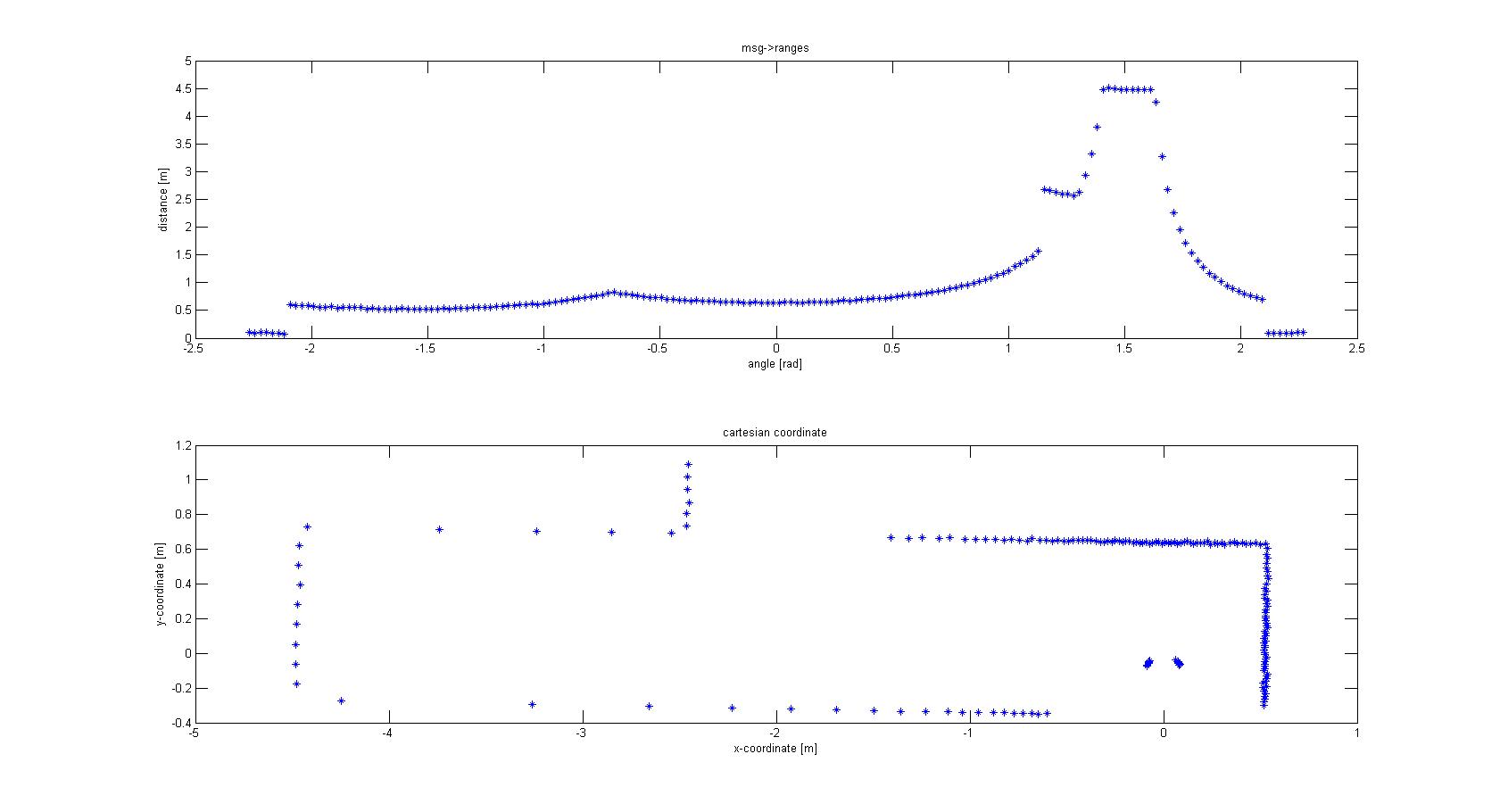
With basic algebra the conversion was made, which is shown in Figure 1.

(Figure 1)

From the Cartesian plot some decisions can already be made. For instance, the data points that are plotted near the robot will have to be removed, since these are laser points that are projected on the robot itself. Furthermore we see a lot of points that are far away from the robot, all at a distance close to 10 meter. This is the maximum range of the laser points on the simulated robot, but on the real robot this might be different and can give a disturbing input. Therefore the data points which are relevant to the robot is limited to a range of TOO_FAR_TO_MAP meters, which is a static float to be fine-tuned to achieve good vision for the robot without large disturbances or processing time (limiting the data points you take into consideration when making decisions can speed up calculation times). Here a value of 1.5 meters was chosen.

The next observation made from the Cartesian plot was that the data from the laser is actually quite noisy, as can be seen in Figure 2. The points do not align in a nice way, which can complicate decision making and mapping. One option is to make a fit over all the data points using basic functions for the walls instead of the points. This is also shown in Figure 2. If you assume that all the walls are straight (at least the walls are not substantially curved) you can use linear functions to represent the walls. If you do this in a correct manner you will only have to compare the robot position and orientation to the linear functions (i.e. only a zero order and first order constant a0 and a1) of these walls. Since you map only walls that are close to the robot this will reduce the input of your algorithms for wall avoidance from the number of laser points (over one thousand for the real life robot) to the first order functions of the walls (which will generally not exceed 8 wall segments, so 16 constants in total). A good motivation to continue developing an algorithm to do this.

(Figure 2)

Mapping Algorithm The fitting of the lines over the data points is done in two steps. First the line start has to be found by making a start line. This start line is MIN_LENGTH_LINE points long. This number can changed be to make the algorithm more robust; here a minimal length of 4 points was chosen. The requirements for the line start are:

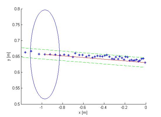
• The points between the first and last point of the start line will have to lie closer to the line fitted between the first and last point of the start than the offset MAXIMAL_OFFSET_EVAL_LINE. This is shown in Figure 3.
• The first and last point of the start line have to lie inside the relevant range of the robot discussed above (not too far and not on the robot itself). However, to avoid that one outlier prevents a line fit, it is allowed that one point falls outside the region of interest. This gives better performance than adjusting the allowed offset since this will give implications when a corner has to be mapped. Therefore all points should lie in between the offsets of the line.

File:Start fit.jpg (Figure 3)

If these conditions are not met, no start line can be made and the search repeats, now with the next data point as starting point. If the start conditions are met, the line between the first and last point of the start line can be appended. This is done by checking if the next data point can replace the end point of the line that is appended. In order to do this, similar conditions have to be met as for the search of the start line, and the point has to lie between the same offset. If the conditions are not met we do not append the line and start searching for a new line with the algorithm described above. However, to map lines at the edge of your region of interest, only if LINE_UNCERT_COUNT points in a row lie outside the region of interest we start looking for a new line (a value of 5 points was chosen). This is done to prevent that if a few points lie outside the region of interest but the wall actually continues the algorithm starts looking for a new line while it can easily continue appending the line it already found. Figure 4 shows the resulting end point of a line.

File:Append line (Figure 4)

With this mapping algorithm the walls are not perfectly mapped. Some walls are split into two lines. One possible solution for this is to change the offset allowed for the points to be added to a line. However, this can cause the algorithm to miss corners easier. This problem was therefore solved by merging lines which clearly fit the same walls. To achieve this the distance between the end point of one line and the start point of the next line have to lie close to each other (maximum of MAXIMAL_DISTANCE_LINE_MERGE meters, an educated estimate of 0.2 m was chosen). Furthermore the slopes of the lines need to be close to each other. One problem that arises is that two lines of a wall parallel to the orientation of the robot can have a very positive slope, or a very negative slope. To account for this fact the slopes are converted to angles relative to the x-axis. If the angles differ less than π/6 rad and the end point and start point are close enough to each other the lines are merged. Since all corners in the maze are roughly π/2 it is not likely that two lines depicting a corner are seen as one wall and merged. Figure 5 shows the merging process.

File:Merge lines (Figure 5)