Embedded Motion Control 2012 Group 5

Group Information

Name	Student number	Build
Fabien Bruning	0655273	Ubuntu 10.10 on Virtualbox in OSX 10.7
Yanick Douven	0650623	Ubuntu 10.04 dual boot with W7
Joost Groenen	0656319	Ubuntu 10.04 dual boot with W7
Luuk Mouton	0653102	Ubuntu 10.04 dual boot with W7 (Wubi)
Ramon Wijnands	0660711	Installed Ubuntu with wubi (included with the Ubuntu CD)

Planning and agreements

Planning by week

• Week 1 (April 23^th -April 29)
  • Install Ubuntu and get familiar with the operating system
• Week 2 (April 30^th - May 6^th)
  • Get the software environment up and running on the notebooks
    • ROS
    • Eclipse
    • Gazebo
  • Start with the tutorials about C++ and ROS
• Week 3 (May 7^th - May 13^th)
  • Finish the tutorials about C++ and ROS
  • Install smartsvn
  • Create a ROS package and submit it to the SVN
  • Read chapters of the book up to chapter 7
  • Make an overview of which elements of chapter 7 should be covered during the lecture
• Week 4 (May 15^th - May 20^th)
  • Make lecture slides and prepare the lecture
  • Finish the action handler
  • Finish the LRF-vision
  • Start with the strategy for the corridor competition
• Week 5 (May 21^th - May 27^th)
• Week 6 (May 28^th - June 3^rd)
• Week 7 (June 4^th - June 10^rd)
• Week 8 (June 11^th - June 17^rd)
• Week 9 (June 18^th - June 24^rd)

Agreements

• For checking out the svn and committing code, we will use Smartsvn
• Add your name to the comment when you check in
• Every Tuesday, we will work together on the project
• Every Monday, we will arrange a tutor meeting

Strategy and software description

Strategy

'Visual Status Report Because a picture is worth a thousand words.

ROS layout

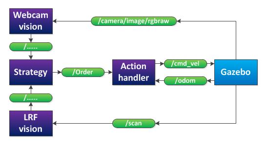
After a group discussing, we decided that our provisionally software layout will be as in the figure below.

The 'webcam vision' node processes the images, produced by the RGB-camera. It will publish if it detects an arrow and in what direction the arrow points. The 'LRF vision' node processes the data of the laser range finder. It will detect corners, crossroads and the distance to local obstacles. This will also be published to strategy. The 'strategy' node will decide, based on the webcam and LRF vision, what action should be executed (stop, drive forward, drive backward, turn left or turn right) and will publish this decision to the 'action handler' node. Finally, the 'action handler' node will send a message to the jazz-robot, based on the received task and on odometry data.

LRF vision

The Laser Range Finder of the Jazz robot is simulated in the jazz_simulater with 180 angle increments from -130 to 130 degrees. The range is 0.08 to 10.0 meters, with a resolution of 1 cm and an update rate of 20 Hz. The topic is /scan and is of the type sensor_msgs::LaserScan. The data is clipped at 9.8 meters, and the first and last 7 points are discarded, since these data points lie on the jazz robot.

The LRF data can be processed in multiple ways. Since it not exactly clear what the GMapping algorithm (implemented in ROS) does, we decided to write our own mapping algorithm. But first the LRF needs to be interpreted. Therefore, a class is created that receives LRF data and fits lines through the data. The fitting of lines can be done in two ways; a hough transform and a fanciful algorithm.

Hough transform

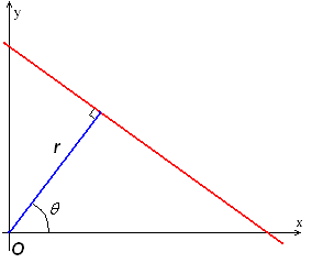
A hough transform interprets the data points of the LRF in a different way; each point in x-y-space can be seen as a point through which a line can be drawn. This line will be of the form [math]\displaystyle{ y=ax+b }[/math], but can also be parametrized in polar coordinates. The parameter [math]\displaystyle{ r }[/math] represents the distance between the line and the origin, while [math]\displaystyle{ \theta }[/math] is the angle of the vector from the origin to this closest point. Using this parameterization, the equation of the line can be written as

[math]\displaystyle{ y = \left(-{\cos\theta\over\sin\theta}\right)x + \left({r\over{\sin\theta}}\right) }[/math]

So for an arbitrary point on the image plane with coordinates ([math]\displaystyle{ x_0 }[/math], [math]\displaystyle{ y_0 }[/math]), the lines that go through it are the pairs ([math]\displaystyle{ r }[/math],[math]\displaystyle{ \theta }[/math]) with

[math]\displaystyle{ r(\theta) =x_0\cdot\cos \theta+y_0\cdot\sin \theta }[/math]

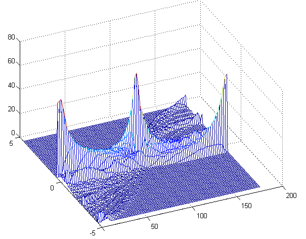
Now a grid can be created for [math]\displaystyle{ \theta }[/math] and [math]\displaystyle{ r }[/math], in which all pairs ([math]\displaystyle{ r }[/math],[math]\displaystyle{ \theta }[/math]) are drawn. Now a 3D surface is created that shows peaks for the combinations of [math]\displaystyle{ \theta }[/math] and [math]\displaystyle{ r }[/math] that are good fits for lines in the LRF data.

In the figure on the right this transform has been performed on the LRF data. Several peaks can be seen that represent walls. The difficulty with this transform is the selection of the right peaks. This can be solved by using some image processing and some general knowledge on the LRF data. This method will however not be used by our group but it is kept in mind in case the fanciful algorithm fails.

Another drawback of this method is that holes in the wall are difficult to detect, since the line is parametrized with [math]\displaystyle{ \theta }[/math] and [math]\displaystyle{ r }[/math] and has therefore no beginning or end. This problem can be fixed by mapping all data points to the closest line and snipping the line in smaller pieces. An advantage is that a Hough transform is very robust, and can handle noisy data.

Fanciful algorithm

We thought of an own algorithm for line detection as well. Since the data is presented to the /scan topic in array of points with increasing angle, the points can be checked individually if they contribute to a line. A pseudocode version of the algorithm looks as follows:

create a line between point 1 and point 2 of the LRF data (LINE class)
loop over all data points
   l = current line
   p = current point
   if perpendicular distance between l and p < [math]\displaystyle{ \sigma }[/math] AND angle between l and p < 33 degrees AND dist(endpoint of l, a) < 40 cm
     // point is good and can be added to the line
     then add point to line
     else false_points_counter++
  end

  if false_points_counter > 3
    then end the line
         decrease the data point index with 3
         create a new line with the first two points
         increase the line index with 1
  end
end loop

LRF processed data

The output of the line detection algorithm is published on /lines, and the map-node is subscribed to this topic.