Mobile Robot Control 2024 Optimus Prime

Introduction

We are Optimus Prime, a team of six members applying various control techniques and coding skills to optimize a robot for restaurant environments. Our goal is to enable the robot to efficiently deliver orders from the kitchen to the tables, even when faced with various obstacles. This project focuses on ensuring precise and reliable performance, ultimately improving service efficiency and the overall dining experience.

Group Members

Caption

Name	student ID
Yuvan Dwaraga	1563793
Wiktor Bocian	1628798
Ramakrishnan Rajasekar	1979027
Ariyanayag Ramesh Skandan	2012618
Abhir Adiverekar	1984136
Suryakumar Hariharan	1974076

Exercise 1 - The art of not crashing

This exercise aims to enhance our understanding of control techniques and obstacle avoidance algorithms.

Simulation of the robot moving

Solution 1

The odometry and laser data were obtained based on the instructions from the manual, enabling the robot to be aware of its surroundings. Although this sensor data does not provide instructions for the robot to stop or go when an obstacle is on its way, a discussion was held to include a constant safe distance value, which ensures that the robot maintains a safe distance from obstacles and avoids collisions. Loops were also introduced as the robot operates to check whether the obstacles are close to the robot or not. Specifically, if an obstacle is detected within a certain range less than the predefined safe distance (0.5 meters) the robot will come to a halt. This algorithm ensures that the robot can navigate in its surroundings safely.

Solution 2

Advancements to the previous solution were made by introducing rotation values and forward motion value to enhance the robot's performance. These values were effective when the obstacle is too close to the robot. The stoppage of the robot comes into play and the rotation values allow it to rotate with movement restriction and later it allows the robot to move in the forward direction with constant units. This approach ensures that the robot not only stops to avoid immediate collisions but also actively seeks a safe route forward. Overall, the combination of a constant safe distance, rotation and forward actions allows the robot to perform more efficiently.

Simulation of the robot movement in x direction

Learnings from solution

The robot's performance in this case was evidenced in both simulation and in practical sessions. Alterations in the code were made so that, in case of the obstacle detection, the robot was made to move in the x direction in adherence to the safe distance.

Practical session

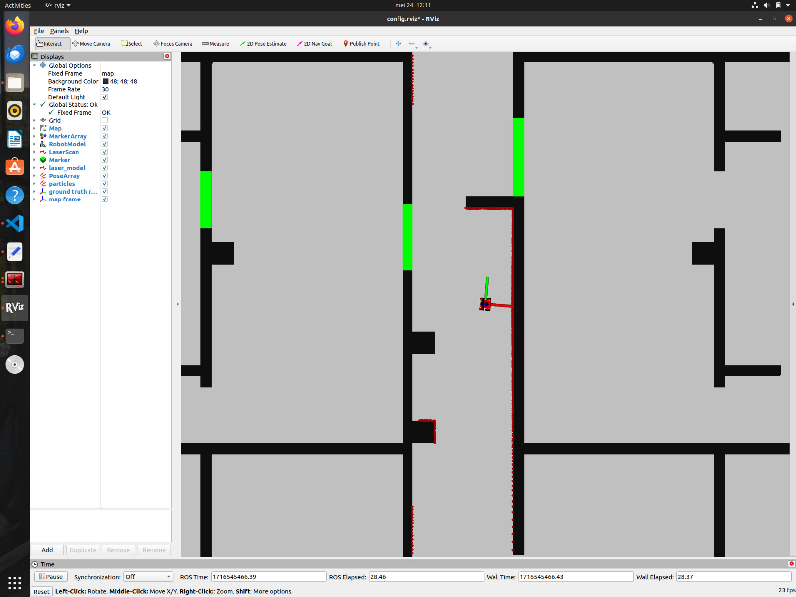
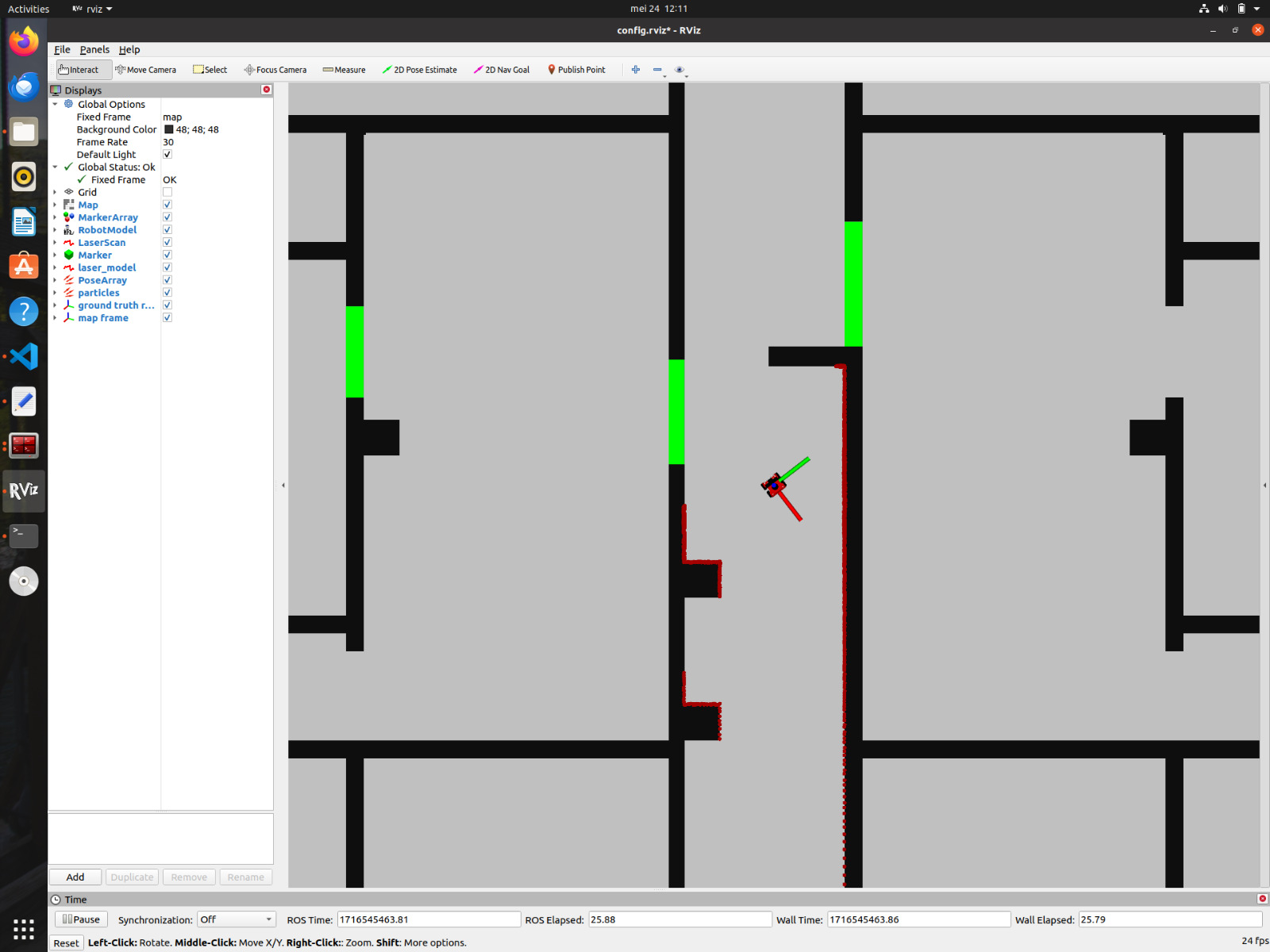
The live testing of don't crash test can be evidenced by accessing the link [1]

Exercise 2 - Local navigation

Artificial potential fields

Motivation

Choosing the artificial potential field (APF) method for local navigation of a robot comes with several compelling motivations:

1. Simplicity and intuitiveness: The APF approach is reasonably easy to grasp and apply. It mimics the environment using attractive and repulsive forces that naturally direct the robot to its destination while avoiding obstacles. This simplicity can be very useful in educational and experimental contexts.
2. Continuous and Smooth Path Generation: This approach creates smooth and continuous tracks for the robot. Because the forces are computed as gradients of potential fields, the resulting motion is smooth, avoiding the possibility of sudden changes in direction that would be difficult for the robot to perform.
3. Scalability: APF is easily adaptable to many types and sizes of settings. The approach may be adjusted to a variety of circumstances by modifying the potential field parameters, ranging from basic inside navigation to more difficult outdoor settings.
4. Combination with Other Methods: APF may be utilized effectively with other navigation systems. For example, it may be used for local navigation inside a larger framework that handles global path planning, integrating the benefits of several frameworks.

Solutions

1. Converting the body fixed frame into global coordinate To implement this a transformedOdometry() function was created which was use to convert the odometry data of the robot into global coordinate.
2. Normalizing the angle The normalize_angle() function ensures that any given angle is mapped to an equivalent angle within the standard range of −π to π radians. This is useful because angles can be represented in multiple ways (e.g., 3π is the same as π), and having a consistent representation simplifies many calculations and comparisons.
3. Calculating attractive forces The attraction_force() function calculates a linear attractive force towards a target position. This force is proportional to the distance between the current position and the target position, scaled by an attraction coefficient.
4. Calculating repulsive forces The repulsion_force() function calculates a repulsive force that acts to push a point (or robot) away from an obstacle when it gets too close. The force is designed to be strong when the point is very close to the obstacle and diminishes as the point moves away, ensuring safe navigation around obstacles.

Learnings from each solution

While the artificial potential field (APF) approach has significant benefits for robot navigation, it also has certain drawbacks, such as the possibility of being caught in local minima or oscillations. To address these concerns, many fixes and improvements to the APF approach have been proposed:

Gradient Descent with Escape Strategies: One typical problem with APF is getting stuck in local minima when the attractive and repulsive forces cancel out.

Solution: Random Walks or Perturbations - By introducing small random movements or perturbations, the robot can escape local minima. To come out of the local minima random perturbations were added in the APF algorithm and it was successful at the end.

Combination with Global Path Planning: Integrating APF with a global path planning algorithm can provide a more comprehensive navigation solution.

Solution: Hybrid Approaches - Finding a rough path with a global planner such as A* or Dijkstra's algorithm, and then using APF for local navigation to fine-tune the path and avoid obstacles.

When tested out with the common settings for the APF it was found that for some maps it was stuck in the local minima, for this different parameters were designed (attractive gains and repulsive gains) for each map and after implementing this strategy the robot was able to function properly for each map efficiently.

Visual representation of sim

1. Map 1 - https://www.youtube.com/watch?v=PWZg0-T9-U8
2. Map 2 - https://www.youtube.com/watch?v=E6Xz24zsPdE
3. Map 3 - https://www.youtube.com/watch?v=ZnRjnttkkrE
4. Map 4 - https://www.youtube.com/watch?v=ERdRPLcliLk

For first three simulation the parameters were the same, but for the fourth simulation the parameters were a bit different.

Pros and cons

Pros

1. Simplicity: The APF approach is straightforward to implement and understand. It uses simple mathematical functions to represent attractive forces towards the goal and repulsive forces away from obstacles.
2. Real-time Computation: APF algorithms are computationally efficient, making them suitable for real-time applications. The computations involved are minimal and can be handled by most modern processors with ease.
3. Scalability: APF methods can be scaled to handle different sizes and types of robots without significant modifications to the algorithm.

Cons

1. Local Minima Problem: One of the significant drawbacks of APF methods is the local minima problem, where the robot can get stuck in a position that is not the goal due to equal attractive and repulsive forces cancelling each other out.
2. Inability to Handle Complex Environments: APF methods may struggle with complex environments with narrow passages or multiple closely spaced obstacles, leading to suboptimal or infeasible paths.
3. Parameter Tuning: The performance of APF methods heavily depends on the tuning of parameters such as the strength of attractive and repulsive forces. Improper tuning can lead to inefficient navigation or failure to reach the goal.

Dynamic window approach

Motivation

Our motivation for choosing the Dynamic Window Approach (DWA) algorithm is that it is one of the most ideal algorithms for local navigation of Mobile Robot Controllers (MRC). DWA strikes a balance between robust obstacle avoidance and efficient navigation. It generates control commands in real-time, which is crucial for dynamic environments. Additionally, it considers the robot's kinematic and dynamic constraints, ensuring that the paths are feasible. The algorithm effectively navigates around obstacles while moving towards its goal, maintaining both precise and responsive movement.

Exercise 3 - Global path planning

A* algorithm

Inflated walls with dilation size equal to 1

Probabilistic Road Map (PRM)

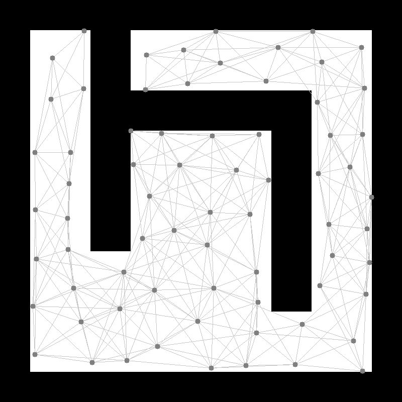
To implement the path planning algorithm a set of the possible paths needs to be created on the map that will be used to find an optimal one needs to be created. To do that the probabilistic roadmap method is used that generates the paths between randomly generated points on the map.

• Wall inflation

Inflated walls with dilation size equal to 2

Because of the size of the robot if the walls on the map are the same size as in reality the chance of the robot clipping the wall or crashing it becomes high since it is not just a point in reality. To avoid that the walls on the map need to be enlarged. To do that dilation on the map image is used. To do that, the map colors are first inverted since dilation works on white parts of the binary image. It is done by specifying the type and size of the Kernel that is used to check if there is a white point inside it and if there is such a point it changes the other ones inside the kernel to this color. For the desired implementation the square kernel is being used since all of the maps mostly consist of straight lines and the size of this kernel can be adjusted by changing the dilation size variable.

After the dilation the map is transformed back to its initial color scheme and examples with different kernel sizes of such operation can be seen to the right.

• Distance from other points

To ensure that points are distributed more evenly around the map the distance between the new vertex and all the previously created ones is being checked. This is done by checking the difference between the x and y coordinates is no smaller than 0.3 m. This ensures that each vertex has a square 0.3x0.3 m area around it of 0.3x0.3 m where there are no other vertices.

• Check for valid edge

To see if the vertex is valid two checks are being done. First to ensure that only the vertices that are relatively close to each other are connected the distance between them is being checked. This is done by computing the absolute value of a difference between the x and y variables of 2 vertices and then taking a square root of a sum of those values squared, which allows us to compute the distance between them in a straight line.

The other check that is being performed is seeing if there is a wall between the two nodes. To do that a line between two points is created using Bresenham's algorithm. It creates all the points along the straight line between two vertices and is used to check if there is a black point along the path. If the line encounters the black point it is marked as invalid and the edge between the two points is not created. This algorithm works by first computing the difference between the x and y position on the line and its final destination. The difference in y is subtracted from the difference in x and doubled to always work on integers, this gives information on how far the generated line is from the ideal straight line between two points. Knowing that if this error is higher than the difference in the y coordinate means that the lines should be less horizontal and the y value needs to be adjusted and the same is done for the x coordinate.

Example

Example of the map created using probabilistic roadmap

To test the algorithm the example map was being used with number of vertices equal to 70, dilation size equal to 2 which means that (5,5) square kernel was used for dilation and maximum distance between two edges of 1 m was created and can be seen on the Figure.