Embedded Motion Control 2014 Group 4

Members of group 4

Khy, R.N.	Norent
Kiriouchine, V.I.	Seva
Kuijk, F.J.M. van	Fransis
Marx, S.	Sanne
Smit, J.	Jorrit

Media

Find videos of the Pico emc04 tests on our Youtube channel.
See here an animated GIF of simulated Pico, where he takes a corner and stops: Animation

Planning

Week 1:
-Introduction Lecture
-Determine course goals

Week 2:
-Install Ubuntu, ROS, fix SVN etc.: get everything up and running
-Finish all tutorials: C++, ROS
-Think of first concepts to tackle the corridor problem
-Implement first concepts: wallfinder, angle/distance controller

Week 3:
-Improve angle/distance controller
-Try to implement holonomic concept
-Meet tutor to discuss problems and project progress
-Perform Pico Test

Week 4:
-[Sanne] Place current functions in seperate .cpp files to allow for parallel updating
-[Sanne]Change the sendVelocity function into a twoPointNavigator function which aims to place pico between two lazer scan ranges+angles given as function input.
-[Fransis]Create a corridorFinder function which identifies the two corners of all corridors large enough for pico to pass through. Discard distant corridors and output two lazer scan ranges+angles of the closest found corridor.
-[Seva]Create a function which decides what points are sent to the twoPointNavigator function based on how close pico is to the side corridor found by corridorFinder , allowing pico to seamlessly switch between navigating the straight corridor and turning into the side corridor.
-[Norent]Change the safety radius into a safety box around pico using the dimensions of pico, create an unStuck function which allows pico to safely move away from any obstacle breaching the safety box.
-Implement a finishedCorridor condition which can detect that pico has left the corridor exit and stops all movement.
-[Pico EMC04]Win the corridor competition.

Concepts

wallFinder
Pico should be able to recognize walls. This can be done by using the Laser Range Finder. The data received from the Laser Range Finder must be filtered to get useful data that can be used by our controller.
From this sensor we receive an array with distances, 270 degrees around Pico. This array is split in half to represent vision on the left and right side. In these two arrays we search for the smallest distance that is greater than 0.15 m (a part of the vision is blocked by Pico him/her/it-self). Finally the angle at wich these distances are with repsect to Pico are calculated. This function thus finds two distances and two corresponding angles.

Angle/Distance controller
When Pico navigates through the corridor the distances found by the wallFinder are controlled to be equal. Besides the distances, the angles at which these distances are detected should be controlled to be zero. When the closest distances left and right of pico are equal and the angles zero, Pico is oriented in the middle of the corridor oriented in the longitudinal direction, which is exactly what we want.

Holonomic movement
At the tutor meeting it became clear that Pico is equipped with omni-wheels which means holonomic movement is possible. Currently the Pico in the simulator has differential wheels. With omni-wheels the distance can be controlled independent of the angle.

Cornering
We should think of how Pico can recognize and take corners.

findExit
We should think of how Pico can recognize the exit of the corridor so that it stops moving.

safetyHitbox
TODO hitbox dimenions (front x side): 2.0e-1 x 1.5e-1.

unstuckSafety
TODO

Implementation

Wallfinder
The wallfinder is called with every lazerscan callback and will return the nearest scanpoint on the left and the nearest scanpoint on the right of pico.

Corridorfinder
The corridorfinder is called with every lazerscan callback and will return the closest corner point of the nearest corridor and the furthest corner point of the closest corridor to pico.
The closest corner is found by looking at the scan data forward of the found wallpoints and determining whether the difference between two subsequent points is large enough. The furtherst corner of the corridor is found by looking forward again past the closest point. When a local minimum is found in the scan distance this is called the furthest corner of the corridor. If the difference between the closest and furthest corner is not large enough for pico to pass through, the corridor is considered a gap.

Masterplanner
The masterplanner determines where to navigate. If the closest corridor corner is very close to one of the points found by the wallfinder, the pico will take the corner using the turnAroundPoint function. If no side corridor is found or the corridor is not close enough, pico will drive forward.
If while taking the corner the closest point on the other side of pico is found at an angle much different from +-90 degrees, the masterplanner knows the pico is mid corner. As soon as the wallfinder again finds the points left and right of pico at the same angle the masterplanner will switch to driving forward.

twoPointNavigator
The twoPointNavigator function will send the velocitys to pico in order to keep pico moving forward between parallel walls. The distance of closest points left and right of pico is controlled to be equal by controlling the linear.y speed. The angle of pico in relation to the walls is controlled by sending an angular.z speed such that the closest point left and right are at and equal angle from the centre of pico.

turnAroundPoint
The turnAroundPoint function will send the velocitys to pico in order to keep pico moving forward while keeping a constant distance to one of the wallfinder points, maintaining this point at a +/- 90 degree angle w.r.t. pico depending on what side the side corridor is.

stopFinal
The stopFinal function is called at each lazercallback to see if the pico has exited the maze using two checks. The first check checks whether all lazer range points are larger than a certain distance. This is the minimum distance pico needs to travel in order for it to consider itself outside of the maze. The second check splits up the lazer scan into 10 sectors, calculating the average distance for each sector. The average distance of each sector has to be greater than a certain (larger than the for the first used check) value. This ensures that the pico will stop close to the maze exit when the majority of the surroundings are very far away.

geometryIdentifier
The geometryIdentifier identifies whether pico is close to any corridors, intersections or junctions, it replaces the corridorFinder for the final test.
The steps taken by the geometryIdentifier are given in pseudo code as:

if (found corridor on the left)

then

if (found corridor on the right)

then

if (left and right corridor are at equal distance to pico

then

if (furthest points of both corridors are wide enough to be a corridor)

then -> Pico has found an intersection

else -> Pico has found a three way left right junction

else -> Pico has found two seperate corridors

else

if (furthest corridor point is much closer than point in front of pico)

then -> Pico has has found a three way left forward junction

else -> Pico has found a corridor to the left

else

if (found corridor on the right)

then

if (furthest corridor point is much closer than point in front of pico)

then -> Pico has found a three way right forward junction

else -> Pico has found a corridor to the right

else -> Pico is in a corridor with no side corridors

Environment Detection

To navigate through the maze, pico should be able to recognize geometries in order to switch to a certain navigating state.
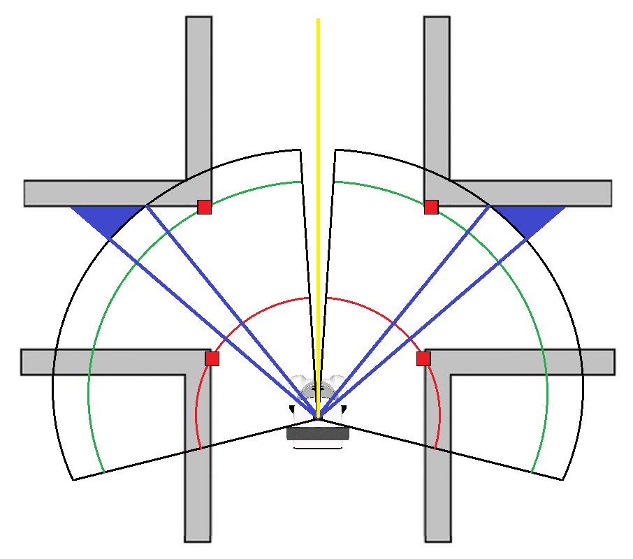
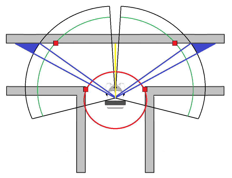
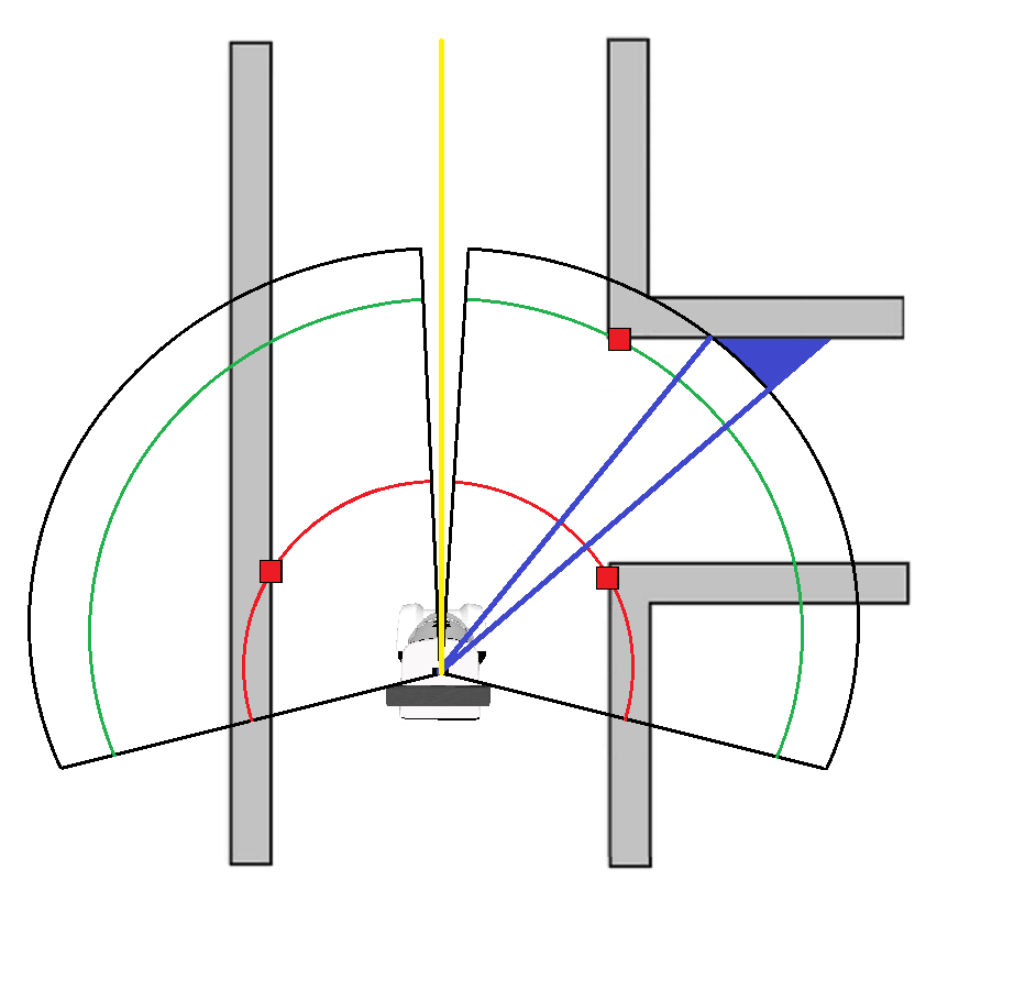
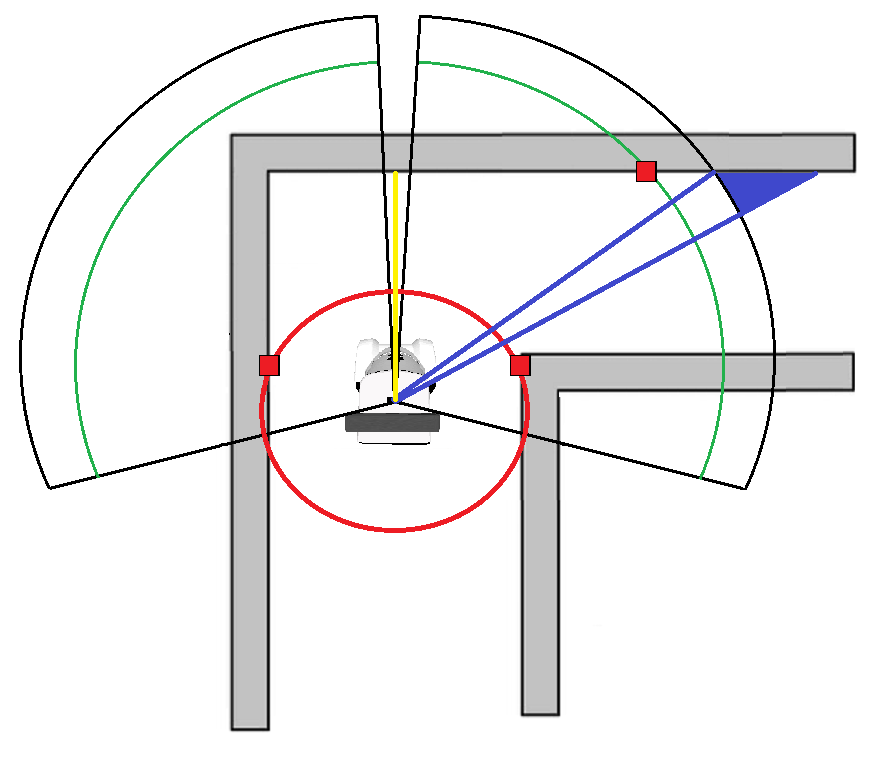
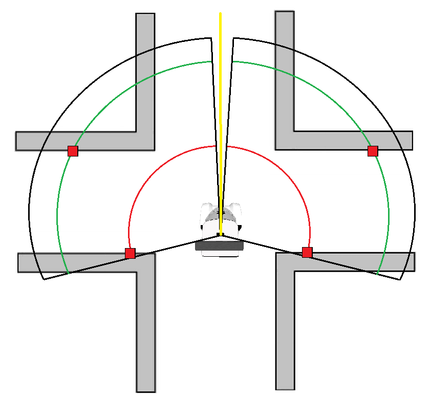
To do this pico’s view is separated in two parts to recognize either a left or a right corner with in the middle a dead zone. This is indicated by a black circular range in the illustrations.
To determine the distance in front of pico a range of points is taken and averaged for robustness, which is indicated by the yellow beam. This distance can be used to determine the difference between 3-way and 4-way junctions, and a corner or a corridor.

The algorithm for either the left or right side is identical and is as follows:

-Start scanning from the left/right side to the middle.
-Find the closest point further than a certain threshold value, indicated by the red circular range. This point is the first corridor point.
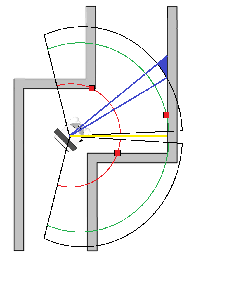
-Continue to scan to find a range of points (indicated by the blue region) that are further than a certain threshold value, indicated by the black circular range.
-If these points are found, continue to scan until the closest point within a certain threshold value is found, indicated by the green circular range. This point is the second corridor point.

4-way Junction
The first corridor points are found on the red circular range, left and right.
A range of points is then found outside the black circular range.
Pico continues to scan to find the second corridor points within the green circular range.

3-way Junction
The first corridor points are found on the red circular range, left and right.
A range of points is then found outside the black circular range.
Pico continues to scan to find the second corridor points within the green circular range.

\

Corridor
The first corridor points are found on the red circular range.
For the right side a range of points outside the black circular range are found. When pico continues to scan it finds the second corridor point on the green circular range.
For the left side the first corridor point is found on the red circular range. A second point isn’t found however because a point within the green circular range isn’t found.
For left corridors the algorithm works exactly the same but on the other side.

Corner
The first corridor points are found on the red circular range.
For the right side a range of points outside the black circular range are found. When pico continues to scan it finds the second corridor point on the green circular range.
For the left side the first corridor point is found on the red circular range. A second point isn’t found however because a range of points outside the black circular range isn’t found.
For left corridors the algorithm works exactly the same but instead on the left side.

Backview Range
In order to detect geometries that are partially behind pico the backview range ensures that this is possible. The corner points in the illustration below are detected correctly.

Switchview
In order to detect new geometries while navigating a current geometry we implemented that Pico’s view switches 90 degrees the moment Pico starts navigating a corner. This can be important when geometries are located very close to each other. While navigating the corner, the view is turned in the opposite direction with exactly the angle that Pico has turned. This is done by using the odometry data. The Switchview ensures that a new geometry can be detected properly. An illustration is given below.

Straight corridor/Dead end

When no left or right corners are found, the geometry is then either a dead end or a straight corridor. This can easily be determined by using the beam

Robustness Features
Corridor width threshold:
To prevent identifying gaps as corners certain robustness-measures are implemented. This can easily be don by calculated the absolute distance between the two points. A corner is only detected if the distance between these two points is big enough for pico to fit through.

Movement

The Movement.cpp file contains a number of functions used to send Twist messages.

NavigateBetweenpoints

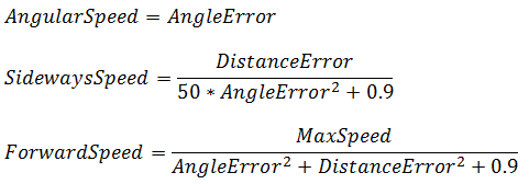
The NavigateBetweenpoints function creates Twist messages that move Pico straight in between two points in space. The difference in the distance to Pico of the two points is saved as the distance error and the difference in absolute angle with relation to Pico is saved as the angle error. Three speeds are then calculated from these errors to ensure that Pico drives straight in-between the points before accelerating.

All these speeds are then capped to the max speed or set to 0 if they are very small (<0.02m/s) to reduce jitter.
Given a large angle error or distance error the forward speed of Pico will be decreased rapidly to ensure that Pico is oriented safely between the two points. If the errors are very low then the equation goes slightly above max speed meaning that after capping the forward speed, Pico is able to drive forward at maximum speed even with small errors in distance and angle measurements.
The sideways speed is controlled linearly with the distance error but since a high angle error means that Pico might be using two points which are not at all on parallel walls the angle error is used to greatly reduce sideways speed until Pico has oriented itself straight between the two points. Because of this structure Pico will, when presented two points to navigate between, first correct for orientation, then for sideways position, and finally start to drive forward at max speed.

ParallelToPoint

The ParallelToPoint function lets Pico drive forward whilst keeping the input point parallel at 90 degrees to Pico at a given distance. A distance error is calculated from the difference between the input point distance and the given distance at which Pico should follow (Usually set at 0.45 m). The angle error is calculated as the difference between the angle the input point has to Pico and 90 degrees.
The speeds are then calculated in the following manner:

As this function is used for driving parallel to walls and to turn around corners with a relatively large radius it is not needed to have fast angular corrections before adjusting the sideways speed. The forward speed is kept the same as in the NavigateBetweenPoints function as this proved to work nicely. All speeds are capped to the max speed and set to 0 if they are very small (<0.02m/s) to reduce jitter.

Maze Tree

The Maze tree is a self-made set of functions used to track the progress of Pico in exploration and to allow a strategy to be implemented. Each separate junction that Pico encounters is saved as a new entry in an array of maze tree elements. These elements contain an ID, parent ID, child ID’s , orientation with respect to the starting orientation and a set of Booleans indicating whether the 4 cardinal directions around it are explored. The animation below shows how the tree is updated as Pico explores a maze. In it Pico uses the strategy of going forward, then right, then left, with respect to the orientation of the maze tree element Pico is in.

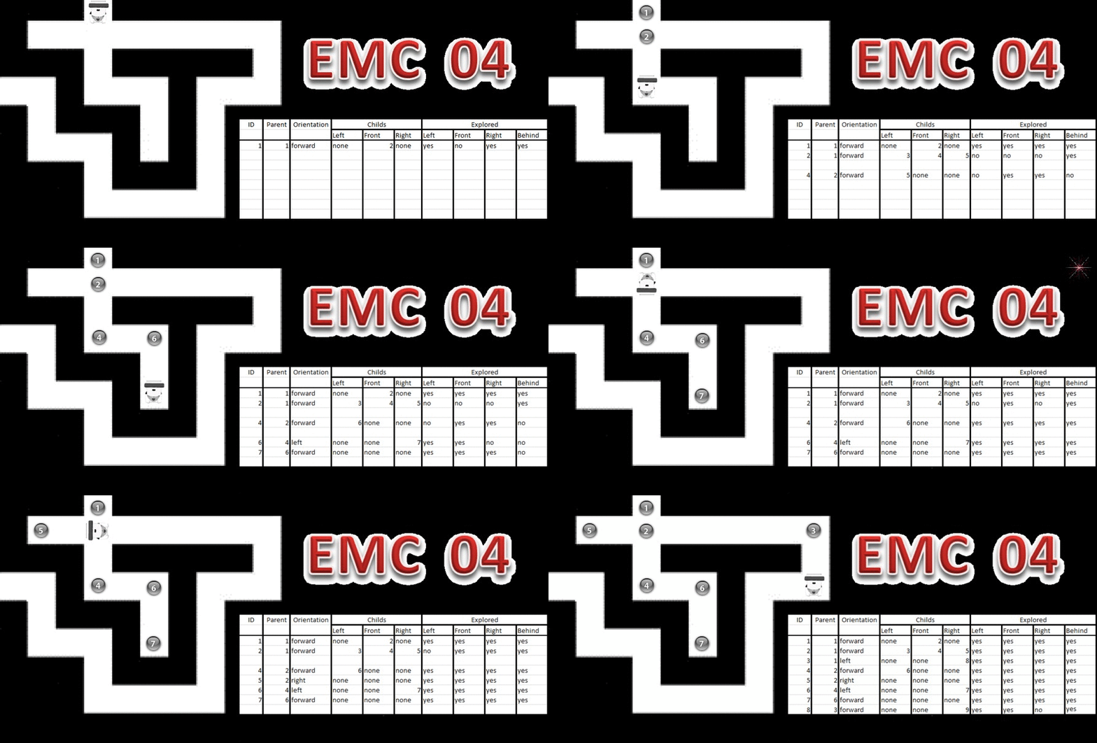
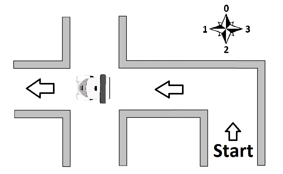
When Pico leaves a tree element through its last unknown direction, that direction is set known in both tree elements it is represented in. The maze tree decides the direction Pico should go, transforming the cardinal directions into numbers this becomes a simple math problem. Forward becomes 0, left is 1, backwards is 2 and right equals 3. The direction Pico should drive in follows from the difference between the preferred strategy direction and the current orientation of Pico + the orientation of the current maze element. If the resulting direction is backwards it is remapped to be forwards. If an arrow is detected it is immediately set as the strategy direction.

Example: Pico is in a 4 way junction that is completely unexplored; the entrance of the 4 way junction is oriented left with respect to the maze start. Pico is also facing left with respect to the maze start. As the maze is unexplored the strategy is to first go forward.

The navigation direction the follows from:

The backwards direction is remapped to forward and Pico knows from this that it should move straight through the 4 way junction. The added 8 is so no negative directions can be the result.

After exploring the forward direction Pico returns to the 4 way junction, Pico is now facing right with relation to the start and wishes to explore the right corridor of the 4 way junction (the corridor facing up in the image) according to the strategy (Forward->Right->Left)

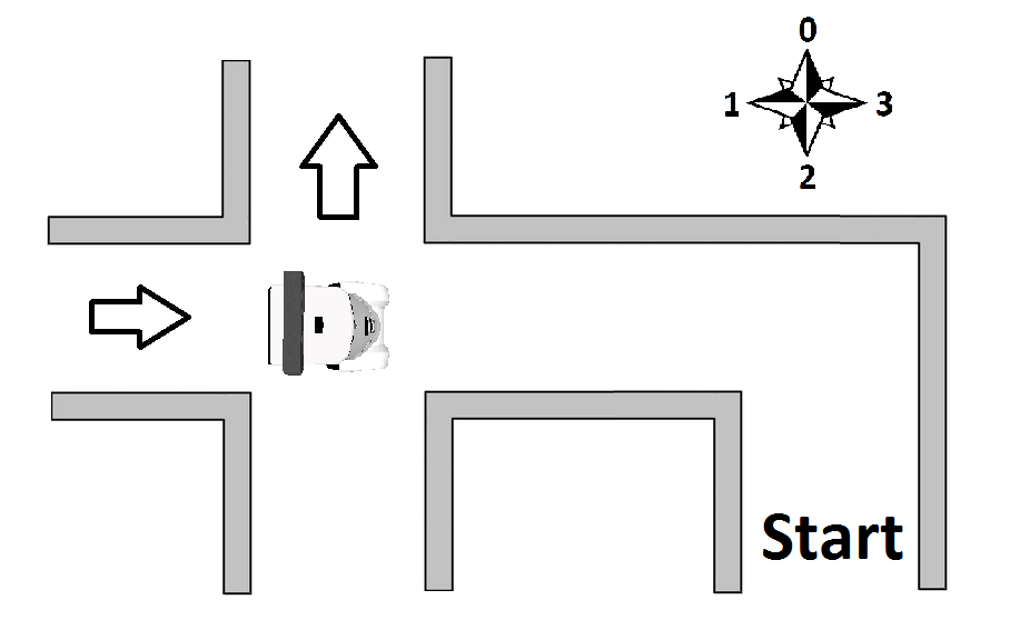
Pico again calculates where to go in the same manner:

Pico therefor knows that it should turn left in order to explore the right corridor in the 4 way junction.

Arrow recognition

Orientation of image recognition techniques (as discussed in lectures)

Three available tools for image recognition:

• Floodfill
• Line detection
• Corner detection

Our initial ideas:

• Line detection: use the position and derivative of the lines to recognize arrow head, tail and direction
• Corner detection: use the point cloud to identify the arrow tail and determine direction by counting nearby points left and right of the arrow tail.
• Floodfill: use enclosed areas on binary image to find arrow candidates, use the area difference left and right to the center point of a valid arrow candidate to determine arrow direction

Two of the initial ideas where discarded:

• Corner detection: The Harris corner detection was thought to be too complicated to implement robustly.
• Floodfill: Does not account for specific geometry, only area and would not be robust enough.

The idea of the line detection algorithm was thought of as the best candidate for a working and robust method of detecting arrows.

Line detection

The main algorithm consists of three main steps:

1. Connect the lines calculated by the Hough transform function in line with each other using their relative proximity and derivative, this new and the original line spaces increase the arrow detection rate.
2. Use the new-line space to see if there exist lines that can be a tail of the arrow and a head of an arrow and how many valid combinations of tail and head can be found.
3. Use most found arrow combination found in part two and take the mode of the past 20 frames as the final output of this arrow detection algorithm for the current frame.

For step 2 the following assumptions were made:

1. The arrows will always be pointing to left or right with a maximum difference of a 20 degree rotation.
2. The maze will not contain too many objects that (that can be interpreted as arrows).
   

Implementation structure:

The three main steps of the detection algorithm are split into the following sub-functions:

1. Image manipulation and line recognition
   1. Convert RGB image to HSV, input: RGB image, output: HSV image
   2. Filter image for red colours in two domains, input: HSV image, output: two red-filtered binary images
   3. Add the two red-filtered binary images into one, input: one red-filtered binary images, output: one red-filtered binary image
   4. Blur the image, input: one red-filtered binary image ,output: blurred binary image
   5. Canny edge detection, input: blurred binary image, output: edge points on new image
   6. Probabilistic Hough line detection, input: edge points on new image, output: vector of line coordinates
2. Arrow Detection
   1. Line joining, input: vector of original line coordinates, output: combined vector of original line coordinates and extended line coordinates
   2. Lines pairing for head, input: combined vector line coordinates, output: integer 1 or 2 as the direction of the arrow or a 0 if no pair is found
   3. Lines pairing for tail, input: combined vector line coordinates, output: boolean whether a tail is found or not
   4. Combining head and tail and calculate arrow direction, inputs: boolean of the tail pair and integer of the head pair, output: number of vaible arrow combinations left or right
   5. Verification by checking the surrounding area of the arrow for other lines, input: arrow lines, output: boolean whether an arrow is verified or not
3. Time mode: Take the most common arrow direction of the past 15 frames, input: past validated arrow combinations, output: arrow directions using three integers

The output of the arrow recognition algorithm is given as integers and is seen in the table below.

message	output
nothing	0
left	1
right	2

The sub-functions of the arrow detection algorithm:

• Converting the RGB image to HSV.
  • The function used is cvtColor which is a part of the open CV library.
• Filtering the image for red colours.
  • The hue in HSV is given in polar coordinates which is representad as an integer value in open CV, this means that red is defined as two integer ranges, the first range in (H,S,V) values as (0, 97, 72) to (13, 255, 255) and the second as (240, 97, 72) to (255, 255, 255). The function inRange is used to produce the binary images.

The two binary images are added using the add function from open CV and the resulting binary image is used to construct lines.

• Blurring the binary image.
  • For blurring the function blur is used with a kernel size of 3, kernel sizes of 5 and 7 where also tried and yielded worse results than a kernel size of 3.

The function median blus was also tested and had no to little preformance difference to the blur function, with kernel sizes 3, 5 and 7.

• Canny edge detection.
  • The function Canny is used from the open CV library with a lower- and upper threshold of 50 and 150 (3*lower threshold), the value 50 is the best value out of 30, 40, 50, 60 and 70. The kernel size is 3.
• Probabilistic Hough line detection.
  • The function used is HoughLinesP, the values for intersect, minimum points and gap points are 10 15 and 5 respectively. This configuration gave small lines, but in large ammounts, which gives high probability of detectiong an arrow where as other configrations gave longer lines but less often which ment that an arrow could not be detected for several frames even though the pico was at a small distance from the arrow.

• Line joining.
  • The HoughLinesP algorithm gives small lines because the binary image is rough and misses pixels, this is a result of the Canny edge detection breaking up edges up to the point where a pixel is missing. To this end a self made line extending algorithm is constructed. The algorithm compares two lines from in their proximity to each other using the end point of the first line and the begin point of the second line, and their relative derivatives.

In the next figure a shematic example is given:

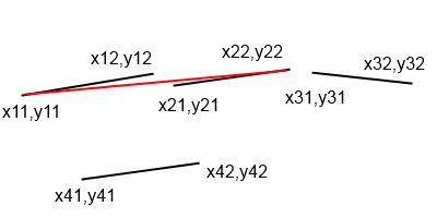
In the figure line 1 is connected to line 2 by checking whether point x12,y12 and x21,y21 are less than 10 pixels appart and whether the difference in the derivative of line 1 and line 2 is less than 0.1, for example: the derivatiove of line 1 is (y12-y11)/(x12-x11) , lines where x12=x11 are discarded as there are no vertical lines in arrows in head nor tail pairs. The longer line is constructed as a line with start point x11,y11 and end point x22,y22 that replaces line 1, note that the original vector of lines is coppied beforehand. This algorithm is then repeated but now for the long line that replaced line 1 and is now compared for the following line, which is line 3, in this case it becomes a longer line with end point x32,y32. For line 4 the difference between points x32,y32 and x41,x42 is too large and the algorithm starts anew with line 2 as the to be extended line. The original lines vector and the long lines vectors are combined into one line vector, which increases the proabillity of finding an arrow. This algorithm has the advantage because not only does it check for gaps between lines as HoughLinesP does, but also checks for relative derivative ranges which negates the faults due to Canny edge detection due to a grainy, pixel missing binary image. The following figure shows the line extender working on a back file:

• Lines pairing for head
  • The head of the arrow determines the direction of the arrow and it consists of two lines at a relative angle range of 45 to 75 degree that are in proximity of each other. The ange is calculated to the horizon of the image using the function atan2 of the derivative. The proximity is defined as the distance of the midpoints of each line which have to be withing 50 pixels of each other in absolute measures and have a minimul distance of 10 pixels. The direction is calculated from the angle of each line in the head pair and the y position is compared of the lines. In the following figure an example is given:

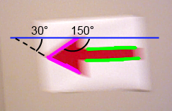
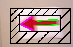
In this example the purple lines indicate a head pair. the top line has an angle of 120 degree and the bottom line has an angle of 30 degree. the relative degree is: (180-angle1+angle2) = (180-150+30) = 60 . The direction is left if the top line has an angle between 130 and 170 degree and the bottom arrow has an angle between 10 and 50 degree, if the bottom line has an angle between 130 and 170 degree and the top arrow has an angle between 10 and 50 degree the arrow is pointing right, if any of these measurements does not suffice this combination of two lines is not an arrow head. In the figure the lines point to the left.

• Lines pairing for tail
  • For two lines to be considered a tail, the lines have to be parallel and in proximity of each other, they may not lie too close to one another . In the previous figure the green lines represent a tail pair. The ange difference is 10 degree, the proximity distances are calculated from the midpoints of both lines, the x distande difference must be at most 50 pixels and at least 5 pixels,

the y distance difference must be at least 30 pixels and at most 150 pixels.

• Combining head and tail
  • The head and tail need to be in close proximity, namely at most 150 pixels apart and the y mid-point position of the tail and head needs to be within 10 pixels of each other. The direction given in the function determining head pairs also needs to be conform with the relative position of head and tail, for example, a left arrow has the head to the left of the tail, meaning the x mid-point position of

the tail needs to be greater than the x mid-point position of the head. If the pair is not conform with any of the aforementioned checks it is discarded.

• Verification by checking the surrounding area
  • The red arrow is printed on a white pice of A4 paper and stuck onto a non-red wall, meaning that around the arrow there should be no lines. For this a safety zone is constructed where the inner region has the highest points from the top and bottom point of the arrow head and the most left and right inner points are determined by the most left and right points of the tail and head, for example an arrow to the left will have a box with most left inner point as the most left head point and a most right point as the most right point of the tail, these edges also have an extra margin of 2 pixels that makes them larger. The top of the outer region is defined as the top inner region plus the longest line of the head pair devided by 3.5 or the longest line of the tail pair devided by 4.5 , this is because the top of the paper does not nescecarily have a non-red wall behind, but may have a red object behind it. The bottom, left and right part of the most outer safety zone points is defined as the inner bound boints plus the length of the longest line in the arrow. In the following figure a safety zone illustrated:

Log

Week 2:
Monday 28-04-2014: Group meeting SEL/SOL
Present: Sanne, Seva, Norent, Fransis

• Installed all software on laptops
  
• Got the svn up and running
  
• Started with tutorials and discussed problems
  

Wednesday 30-04-2014: Meeting SEL/SOL
Present: Sanne, Fransis

• Finished tutorials
  

Friday 02-05-2014: Meeting OGO 2
Present: Sanne, Seva, Norent, Fransis

• Created concepts: wallFinder, angle/distance controller, exitFinder, Cornering
  
• Implemented the following concepts: wallFinder, angle/distance controller:
  
• Pico now can detect walls and navigate through the corridor, not controlled optimal yet

Week 3:
Wednesday 07-05-2014: Group meeting OGO 18
Present: Sanne, Seva, Norent, Fransis

• Held first tutor meeting with Sjoerd
  
• Created holonomic concept
  
• Prepared for real world Pico test
  

Thursday 08-05-2014: First experiment with Pico
Present: Sanne, Seva, Norent, Fransis

• Preparation for the experiment by reviewing the tutorials and our work
  
• Tested code on Pico
  
• Saved logfiles
  
• Observed Pico's behaviour as expected:
  
  • Safety precautions work
    
  • Speed limits work
    
  • Robust for gaps in wall
    
  • Robust for small corridors (width: 8e-1 [m])
    
  • Robust for non-straight corridors
    
  • Unable to make the turn for the corridor contest
    
• Measured Pico rectangular hitbox:
  
  • front: 1.5e-1 [m]
    
  • side: 2.0e-1 [m]
    
  • Made videos of experiments (uploaded soon™)

missing a part

Thursday 28-05-2014: Work session
Present: Sanne, Seva, Norent, Fransis

• Worked in seperate groups on decision making and arrow recognition
  
• Meeting with Sjoerd
  

  Time Table

  Overview of time spent per group member

  	Lectures	Group meetings	Mastering ROS and C++	Preparing midterm assignment	Preparing final assignment	Wiki progress report	Other activities
  Week_1_Norent	2
  Week_1_Seva	2		6
  Week_1_Fransis
  Week_1_Sanne	2		2
  Week_1_Jorrit
  Week_2_Norent	2		6
  Week_2_Seva	2	6	2
  Week_2_Fransis	2	4	6
  Week_2_Sanne	2	6	4			0.5
  Week_2_Jorrit
  Week_3_Norent		1	3	3			1
  Week_3_Seva	2	12
  Week_3_Fransis	2	8
  Week_3_Sanne	2	12
  Week_3_Jorrit
  Week_4_Norent		13					2
  Week_4_Seva		15					2
  Week_4_Fransis		15
  Week_4_Sanne		15					2
  Week_4_Jorrit
  Week_5_Norent		8
  Week_5_Seva
  Week_5_Fransis		20
  Week_5_Sanne
  Week_5_Jorrit
  Week_6_Norent
  Week_6_Seva
  Week_6_Fransis		20
  Week_6_Sanne
  Week_6_Jorrit
  Week_7_Norent
  Week_7_Seva
  Week_7_Fransis		18
  Week_7_Sanne
  Week_7_Jorrit
  Week_8_Norent
  Week_8_Seva
  Week_8_Fransis		24
  Week_8_Sanne
  Week_8_Jorrit
  Week_9_Norent
  Week_9_Seva
  Week_9_Fransis		24
  Week_9_Sanne
  Week_9_Jorrit
  Week_10_Norent
  Week_10_Seva
  Week_10_Fransis		20
  Week_10_Sanne
  Week_10_Jorrit