Mobile Robot Control 2021 Group 5
Team members
Jaap van der Stoel - 0967407
Roel van Hoof - 1247441
Remco Kuijpers - 1617931 - r.kuijpers1@student.tue.nl - 0611135100
Timo de Groot - 1629352 - t.d.groot2@student.tue.nl
Roy Schepers - 0996153 - r.j.m.schepers@student.tue.nl - 0631329826
Arjan Klinkenberg - 1236143 - a.m.klinkenberg@student.tue.nl
Design document
- The Design Document: File:Design Document Group 5.pdf
Escape Room Challenge
Strategy
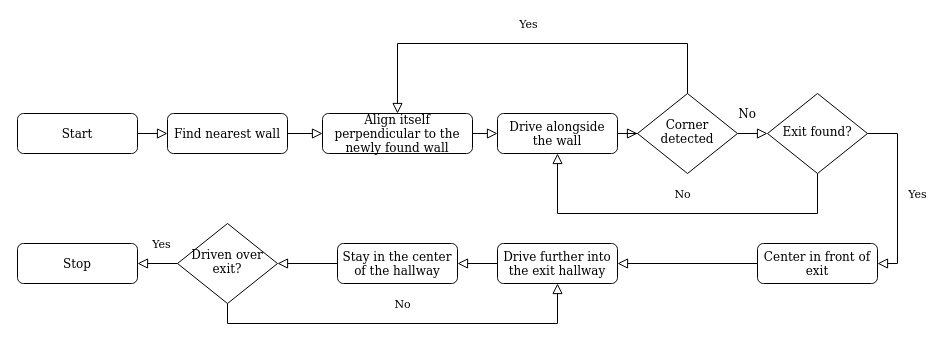
At The start of the escape room challange, the PICO searches for the closest wall. It then drives to this wall and allignes itself sideways to the wall. The PICO then drives straight ahead until either another wall, or the exit, is detected. In the first case the PICO rotates to align itself with the new wall and drives forwards again. In the second case the PICO rotates to align with the exit and then drives through the corridor of the finish line. A graphical representation of the strategy can be seen in Figure 1.
Implementation
Starting and finding nearest wall
At the start of the run the PICO will turn around 360 degrees to look for the wall which is closest to the PICO. When it has identified this direction it will turn to this direction and drive straight to this wall until it is 0.4m apart from the wall.
Aligning to the walls
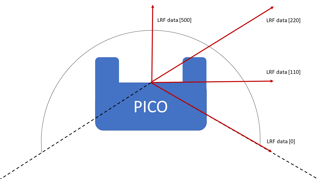
As PICO has driven to a wall, it has to align itself to the wall. To do so, laser range finder data is used. The laser range finder should return the same distance at coefficients 0 and 220 for PICO to be alligned to the wall. In Figure 3 it can be seen how the laser range finder coefficients are defined. As previously mentioned, PICO has driven to a nearby wall. Afterwards, it starts rotating quickly until the laser range finder data of coefficients 0 and 220 ratio is less than 0.2. Then it starts rotating slowly, until the laser range finder data of coefficients 0 and 220 ratio is less than 0.04. If this is the case, it is assumed PICO is alligned to the wall.
Driving along the wall
Now that PICO has aligned itself to the wall, it is going to drive alongside the wall. By doing so, multiple things can be sensed by the laser range finder. First off, if LRF data [500] senses a wall nearby, PICO stops, turns approximately 90 degrees, aligns itself to the wall, and starts to drive forward again. Secondly, if the ratio between LRF data [0] and [220] becomes too large, it is probable that a gap in the wall PICO is following is found. As a gap is found, PICO stops and is going to execute its exit procedure.
Exiting The Room
When PICO has identified an opening in to a wall it will start the exiting procedure. This will be done by turning around 90 degrees in the direction so that it faces the opening. It then drives sideways up to the point that it is in the middle of the exit corridor. PICO needs to drive forward and checks if it is not going too close to the wall.
Centering in the Halway
For the escape room challenge the decision is made to make the PICO center in the exit hallway. The idea is that this maximizes the distance to the walls and thus minimizes the chances of a collision. In applications where the robot may need to navigate a corridor where other dynamic objects are present, such as humans, it may be desirable to make the PICO drive on one side of the hallway. However, this is not the case for this challenge and thus a more robust solution is better. Centering the PICO in the hallway is accomplished by measuring the distance to the walls at a pre-determined angle to the left and right from the normal direction of the PICO. On each side of the normal 20 datapoints are measured in a band around the set measurement angle α, as shown in the Figure 4. The average of the 20 measured distances is then calculated to mitigate the affect of noise on the measurement. The distance to the left and right are then compared to each other and as long as they are within a certain range the PICO is centered. If they are not within the range the PICO moves either to the right or to the left to compensate. While the PICO is moving left or right it also continues to drive forward, in order to move as fast as possible.

Results Escape Room Challenge
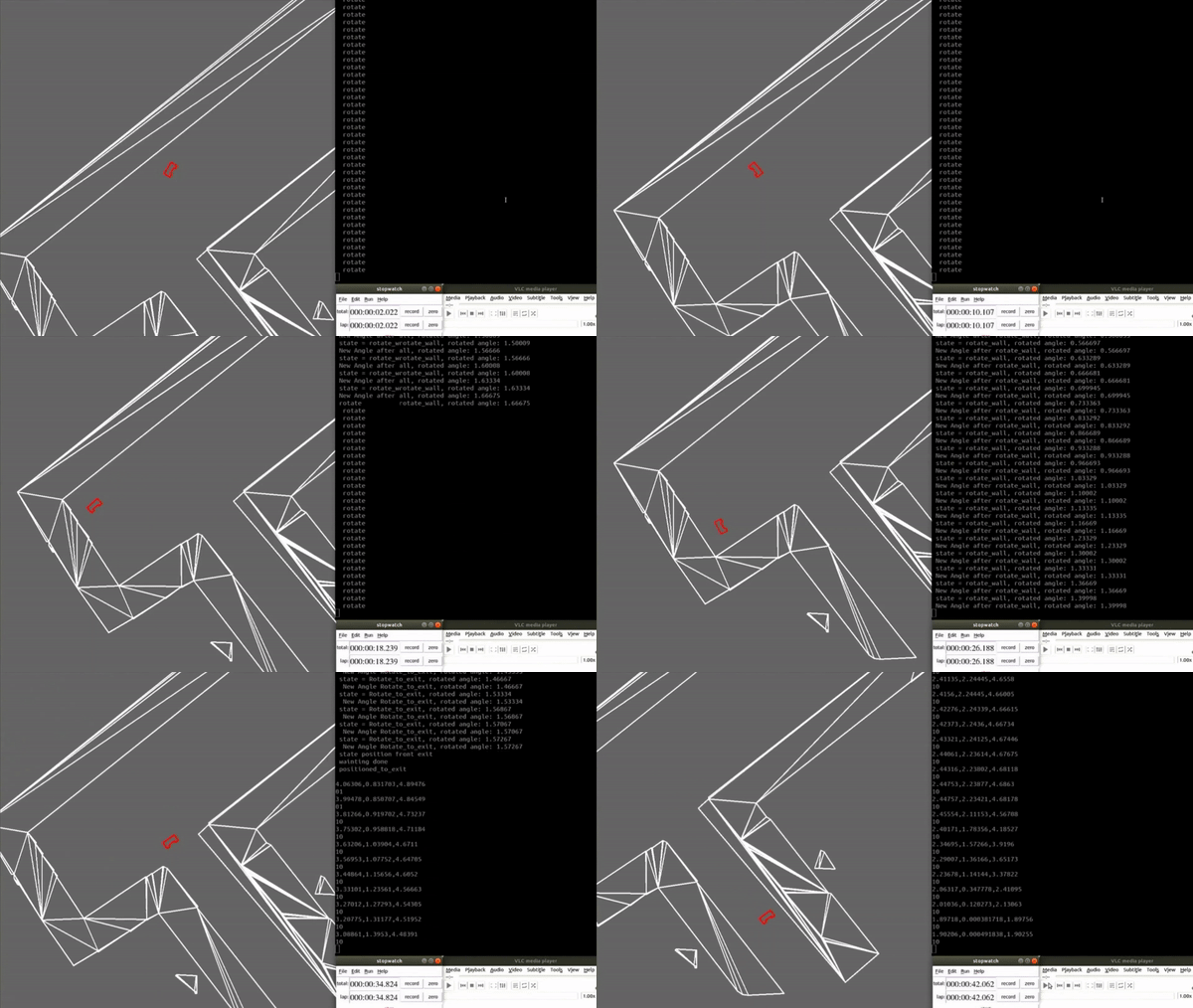
The escape room challenge is successfully complete and the PICO has escaped within 42 seconds, as can be seen in the video bellow.
Improvements
A few improvements can be considered and may aid in designing better software for the hospital challenge. One possible improvement is to decide, when aligning to the wall, what direction to turn would be the fastest. [add more improvements]
Hospital challenge
Strategy

The overall strategy can be seen in Figure 5. However, the localization procedure and path planning itself need to be investigated so the best option in the hospital challenge will be used.
Path planning
Artificial potential field Algorithm
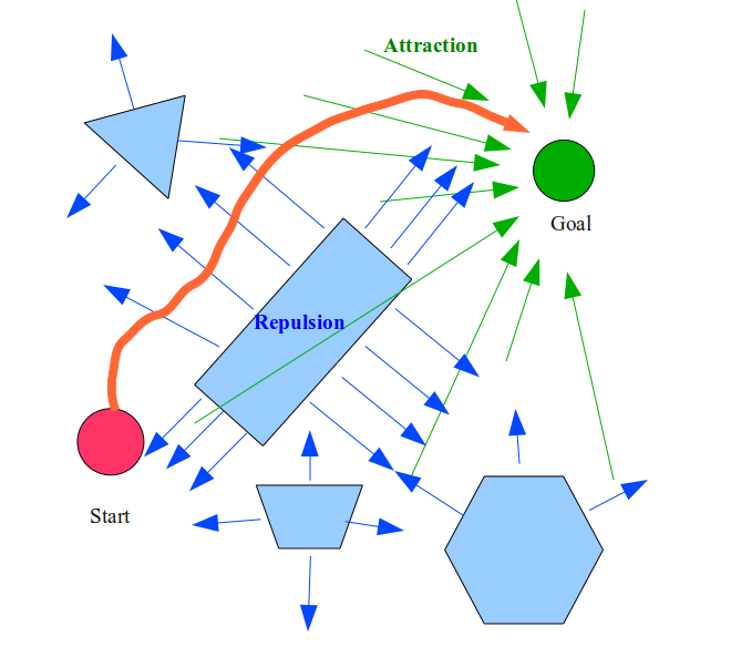
Robot planning by means of the artificial potential field algorithm acts similarly as a charged particle where the robot is attracted to the target and repelled by obstacles as one can see in Figure 6.
The control input uses the attraction and repulsion factor to calculate the control input and the inputs are the weighted sum of both. These weights can be adapted to the specific needs of the path planning case. One pro of the artificial potential field algorithm is the computational power necessary to plan a path. Additionally, the planned path can be smooth and realistic. However, a con of the artificial potential field algorithm is the possibility to get stuck in a local minimum.
Dijkstra's algorithm
The Dijkstra's algorithm is an algorithm for finding the shortest paths between nodes in a graph. There are many variants of this algorithm, but the more common variant uses a fixed single "start" or "source" node and finds the shortest path to the "end" node producing a shortest path three. It does this with a priority que which sorts the possible paths by the sum of their weights. Factors of the weights are most commonly the distance in constant velocity maps, but when taking the example of a route planning algorithm for maps the type of road or even traffic jams can be taking into account. The speed of the algorithm described in the big O-notation is equal to O := (|E|+|V|log|V|), where |V| is the number of nodes and |E| is the number of edges. This efficiency can be achieved by using a Fibonacci heap min-priority queue. This is asymptotically the fastest known single-source shortest path algorithm for arbitrary directed graphs with unbounded non-negative weights.
It is quite hard to explain this algorithm without visalization, but what is basicly does is:
- You create a map with different nodes and vertices for all the junctions of the possible routes. The vertices receive a certain weight factor which is equal to the distance in our case.
- A "start" and "end" node needs to be given from where the algorithm starts finding the shortest path to the end node.
- The algorithm tries every possible direction it can go to from the start node and stores them in separate branches.
- From the first branch it does the same thing, but adds up the weight to the first branch which eventually leads to paths which have a lower value and thus a shorter distance.
- It sorts the these paths again by their weight.
- It keeps on doing this until one path reaches the end point and no branch has a weight lower value than this path.
- The algorithm reroutes this path and gives this as the fastest path. \n
A* search algorithm
This algorithm is an extension on the Dijkstra's algorithm. It is used in many fields of computer sciences due to its completeness, optimality and optimal efficiency. One major drawback is its O(b^d) space complexity as it stores all generated nodes in memory. Therefore, it is mostly outperformed by other algorithms due to memory capability and because with most algorithms can be pre-processed which makes them more efficient. This is due to the fact that the A* approach needs to examine all equally meritorious paths to find the optimal path. However, this can be speed up by relaxing the admissibllity criterion, which means nothing more than that we accept that the found path is not the most ideal one, but is compuationally more efficient.
Visibility graph
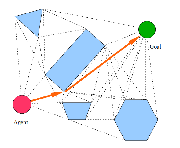
The visibility graph creates a path by connecting all points on the convex hull of the polygonal obstacles to each other and the agent and goal. Then the shortest path is calculated which is the generated path. To accommodate for the width of the PICO, the PICO can be modeled as a disk and the edges of the obstacles should be offset by the radius of the disk.
Pro’s:
- Guarantees to find the shortest path.
Con’s:
- Takes a lot of computing power.
- The graph needs to be recalculated when new objects are discovered.
- Doesn’t handle dynamic obstacles well.
Voronoi diagram
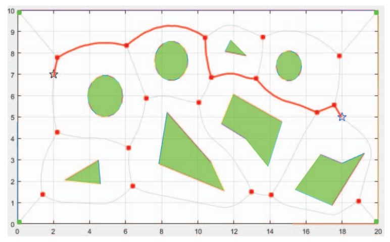
The Voronoi diagram creates lines that are equidistant from al neighboring obstacles. These lines and their connections create the graph of all possible routes through the space. An algorithm like Dijkstra’s algorithm can be used to find the optimal path [3].
Pro’s:
- Creates the most safe path, since the distance to obstacles is maximized.
- The map can be locally updated when dynamic changes are measured.
- Fast algorithm.
- Creates smooth trajectories.
Con:
- this method doesn't guarantee the optimal path.