Mobile Robot Control 2020 Group 10
Team members:
Arend-Jan van Noorden (1378147)
Sjors Boutkan (0938234)
Jeroen van Meurs (0946114)
Koen van Gorkom (0954964)
Friso Buurman (0906665)
Escape Room
Design Document
The design document of group 10 can be found here.
Strategy
Solving the escape room is quite simple: find the corridor and drive through it. This document givesan overview of the system being build to solve this task.Finding the corridor is done by detecting the two outside corners marking the start of the corridor.Since the room is square, no other outside corners will be present in the environment. If these cornerscan’t be found from PICO’s initial location, it’ll follow the walls of the rooms clockwise, until thecorridor (outside corners) are encountered. The corresponding state diagram is shown in Figure1.1. The movement and navigation will be done using set-points and a potential-field algorithmpreventing PICO from hitting any obstacles or walls.
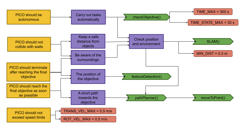
Requirements and Specifications
| Requirements | Specifications |
|---|---|
| PICO should not bump into walls | PICO's measurements are 0.41 m in width by 0.35 m in length |
| The free radius around PICO should be at least 0.21 m | |
| PICO cannot exceed speed limits | Maximum translational velocity is 0.5 m/s |
| Maximum rotational velocity is 1.2 rad/s | |
| Since PICO will be autonomous, it should be aware of its surroundings. | PICO should have an accurate map of its surroundings. |
| LRF range is between 0.01 m and 10 m. | |
| LRF FOV is from -2 to 2 rad, measured over 1000 points of equal increments. | |
| PICO should terminate when the final objective is reached. | PICO should come to a stop after it has crossed the finish line. |
| PICO should reach the final objective as soon as possible. | PICO should cross the finish line within 5 minutes. |
| PICO should not end up in a live lock state. | PICO should not keep repeating one action for over 30 seconds. |
| PICO should not end up in a dead lock state. | Careful coding has to be done to have no dead lock states. |
Components and Functions
Basic architecture of robot code:

All functions need to be run based on a Finite State Machine. As with sensors, all data has noise so these data streams need to be filtered.
The tasks of each component can be divided in several functions each with a specific subroutine.
World model
The world model stores the information gathered by the components and distributes this information to the other components. The information consists of:
- A map of the surrounding area.
- A list of found features.
- The current and previous state.
- The next position to travel to.
The world model contains no functions because the world model is only used to store the world data, so there are no active subroutines present.
Plan
The plan component uses data from the world model to determine the next position PICO needs to go to. It thereby also check if the objective is met.
- checkObjective()
The checkObjective function is the supervisor of the complete system. It controls/executes the states as defined in figure \ref{fig:state-machine} and executes the strategy as described in \ref{sec:strategy}. It will also check for failure of the system by identifying incorrect states, e.g. not moving for a set amount of time, following a wall for too long or having made a complete loop of the room without finding the corridor.
- pathPlanner()
The plan component contains the path-planner function, this functions is responsible to define the setpoints for PICO. These setpoints will be determined based on the state machine and the world model.
Control
The control component makes sure PICO moves along the planned path.
- moveToPoint()
The move to point function will be used to move PICO to the set point generated by the path planner. To prevent that PICO will hit the wall, the world model will be used to determine the trajectory from the current position of PICO to the set point.
Monitoring
The monitor component will try to identify features from the world model data.
- featureDetection()
To determine the corners and walls of the maze the feature detection function will be used based on the world model data.
Perception
The perception component will gather the sensor data, clean it and update the world model with it.
- getLaserData()
To acquire the data points of the laser sensor, the get laser data function will be used. The gathered data will be preprocessed to filter out the disturbances. The processed data will be written to the world model.
- getOdomData()
The odometry date will be read out with the getOdomData function. This date will be written to the world model.
- SLAM()
The gathered data from the laser and odometry sensors will be used to generate a map of the environment using Simultaneous Localization and Mapping (SLAM)
- UpdateVisuals()
A window will be opened that shows all the detected features and the path that PICO is going. This function will update that window
Interfaces
All components interface with the world model, getting data required for their functions and setting data created to be used by other components. The world mode is the central data store. This can also be seen in figure Figure Boven. Differences between the the proposed system and the system originally shown in [1], is that there are no interfaces between the 'resources' and 'capabilities' and the world model. The world model will not be able to get it's own data or control the motors of the system. The interface to the sensors will be through the perception component and the controlling of capabilities will be done by the control component.
Challenge result
Sadly we did not manage to get out of the escape room, below we will discuss why and how we solved it.
Main
After the Maze challenge we analyzed which part of the main program caused the failure which lead to the the wall collision. The problem occurred in the corner detection function, which resulted in the interpretation of a inside corner as an outside corner. The planning algorithm used this corner as target position to search a second outside corner, and let the robot drive to this corner. With the absence of a potential field algorithm, the robot was able to drive through the wall.
The main program for the maze challenge is using the state machine as shown in the Components and functions paragraph, in the following paragraphs is the robot behavior at each state described.
- ORIENTING
In the first state the robot will turn to check if it can see a door or a outside corner. A door is defined if there are two outside corners within 0,5 m and 1,5 m from each other, or a outside corner and a wall within the same range as with the outside corners. If the robot is not able to find a door from its initial position, then there will be searched for a single outside corner. When there is no door or outside corner found then the robot will search for the closest wall to follow.
- SEARCH_FORWARD
If the robot cannot detect any features in the orienting state, then the robot will drive straight forward in the same direction as the initial orientation.
- ALIGN_TO_WALL
When multiple walls are detected the closest wall is determined, the angle between the wall and the robot will be computed to determine the rotation direction. When the robot is aligned within +/- 3 degrees the state will be set to FOLLOW_WALL.
- FOLLOW_WALL
The robot will follow the wall at 20 cm distance till a door or outside corner is found, if this is the case the state will be set to GOTO_DOOR or SEARCH_DOOR. Otherwise the robot will follow the wall if a second wall in front of the is found, when this second wall is closer by then the first wall the ALIGN_TO_WALL state will be called again.
- SEARCH_DOOR
If one outside corner is found a way point will be set 25 cm from the x and y direction with respect of the corner, with this way point there can be guaranteed that the robot will not collide with the wall. When the robot is at this position and the second outside is still not found it will to ORIENTING again, otherwise the robot will be set GOTO_DOOR.
- GOTO_DOOR
When the door is found the planning script will place a way point 25 cm in front of the midpoint of the door, if the robot is at this location the robot will be set to the DRIVE_THROUGH_DOOR state.
- DRIVE_THROUGH_DOOR
In this state the robot will drive to the way point 25 cm in the middle the door, when the robot loses the door the DRIVE_THROUGH_CORRIDOR state is set.
- DRIVE_THROUGH_CORRIDOR
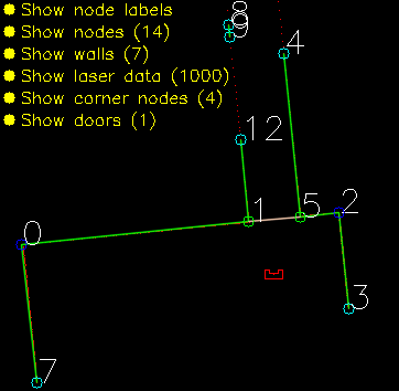
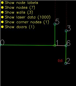
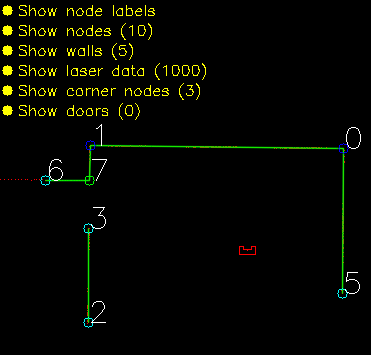
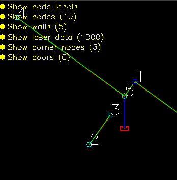
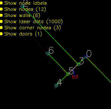
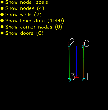
To complete the maze a way point is set in the middle of the furthest corridor walls nodes. To determine the corridor walls there is checked if the walls are parallel to each other, if the perpendicular distance is between the 0,5 m and 1,5 m and if at least two wall nodes can be projected on the other wall to check if the walls are not after each other. When the robot is at this way point the robot has exited the maze and the state will be set to COMPLETED. Below there is shown that the robot is executing SEARCH_DOOR, GOTO_DOOR and DRIVE_THROUGH_CORRIDOR.
Backup

The backup was a simple wall following algorithm. Initially, Pico will drive forwards until it encounters an object in front. Next, Pico will turn 90 degrees to the right. Then, as long as Pico's left side is obstructed, the wall will be followed while making adjustments to align with the wall and not strafe too close to the wall or too far away from the wall. Again, when the front is obstructed as well, Pico will turn 90 degrees to the right and the next wall will be followed. When a gap at the left side is detected, Pico will move forward a little bit, turn left and drive forward into the corridor. If the senses a object in front, Pico will know the opening was only a small gap and not the corridor, in this case Pico will rotate right and continue following the wall.
Unfortunately, the backup attempt failed as well. The problem Pico encountered during the challenge was an edge case which unfortunately did not result in a correct execution of the algorithm. After finding a wall at the front, Pico turned 90 degrees to the right. After the turn all sides were 'free', meaning that Pico thought he was next to a corridor. After turning left it noticed that its front was free and its left side was not. This triggered the state machine to believe it was in the corridor. When the state machine enters this state, the only possible state is the finished state. So after driving through the wall, all sides of Pico were 'free' again thus entering the finished state. Pico drove through the when it thought it was in the corridor. This is because of the specific laser beams that Pico uses for the collision detection. Pico checks three sides, using ten laser beams per side. The front side is the actual front of Pico. The right and left side however, are about 45 degrees from the front instead of 90. Since the actual side of Pico was not monitored, Pico thought he was still some distance away from the wall.
After the challenge a little time was spend to improve the behavior of the wall following algorithm. To this end, the hard 90 degree turns have been replaced by an alignment check and the collision detection was changed that the actual right and left side of Pico are measured. When an obstructing in front is detected, Pico rotates until the obstruction is not visible anymore and the left side is aligned to a wall. This is checked by comparing the ranges of a subset of the of the LRF to the left of Pico. When the ranges are about equal, Pico is aligned. With this improvement, Pico was able to reach the actual finish of the Maze Challenge.
Hospital challenge
The hospital challenge is based upon a real-life scenario where a PICO robot can assist with tasks in the hospital. The goal of the robot is to visit different cabinets to gather or deliver medicenes for example. This process should be executed as smooth, fast and safe as possible. The main challenges which arise are the planning and the path of the robot, which is unknown before the start. The robot should be able to determine its path’s on the run. The robot should also be able to robustly navigate through the hospital. Imperfect walls, static and dynamic clutter, such as garbage bins or people, and wheelspin are all present in practice, while these are not necessary present in a perfect simulated environment.
Strategy [Sjors]
In order to succesfully complete the given task, the structure of the code which runs the robot must be well designed, structured and intuitive. The code is divided into multiple components, which all serve a different task.
[#World model|World model]] is used to store the information of the map and the sensors in two maps, a global map and a live map. The information is read from and written to this world model.
Planning is used in order to plan an optimal path through the map, which can change when clutter or closed doors are encountered.
Control focuses on the actuation of the robot itself.
Monitoring is a big component which takes all the perception data, and uses it to determine the position of the robot, the live map, and ???
Perception is the component which translates the raw sensor data to usefull information.
Statemachine is the brain component of the robot, and decides which steps need to be undertaken in order for the robot to complete its task.
The User interface is used in order to visualize the maps, the robot and its behavior, and can give tremendous insights during testing and execution of the tasks at hand.
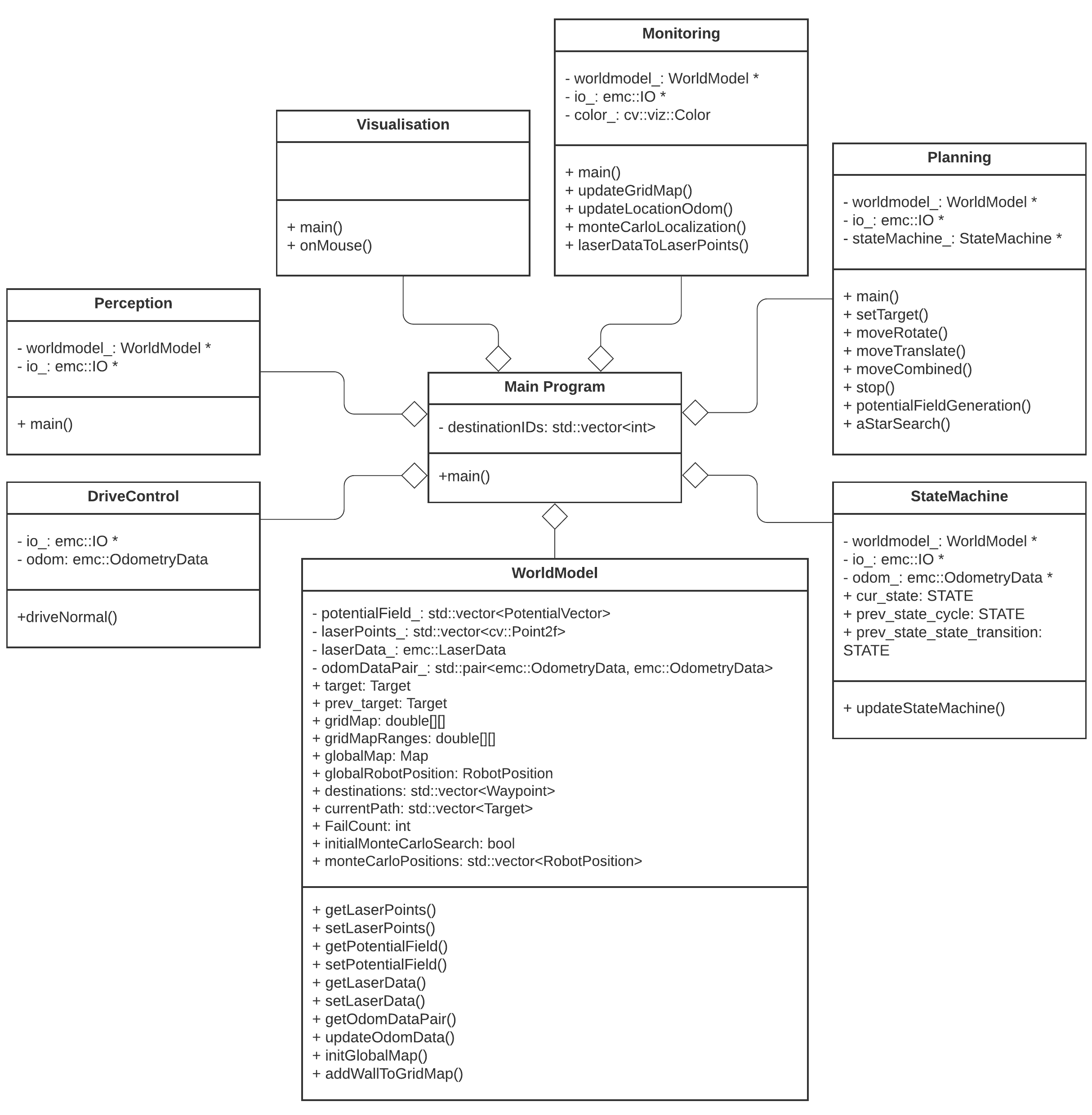
The program written has been designed in a way such that the semi-independent components all work together. Some of these even work in parallel to improve qualitative performance. In the following sections, these different components and their interactions will be dissected and explained. Below, a UML class diagram can be seen showing the different components and their most important member attributes and methods.
Meer uitleg over de UML Class Diagram?
Clicking this thumbnail will show the full sized version of the image.
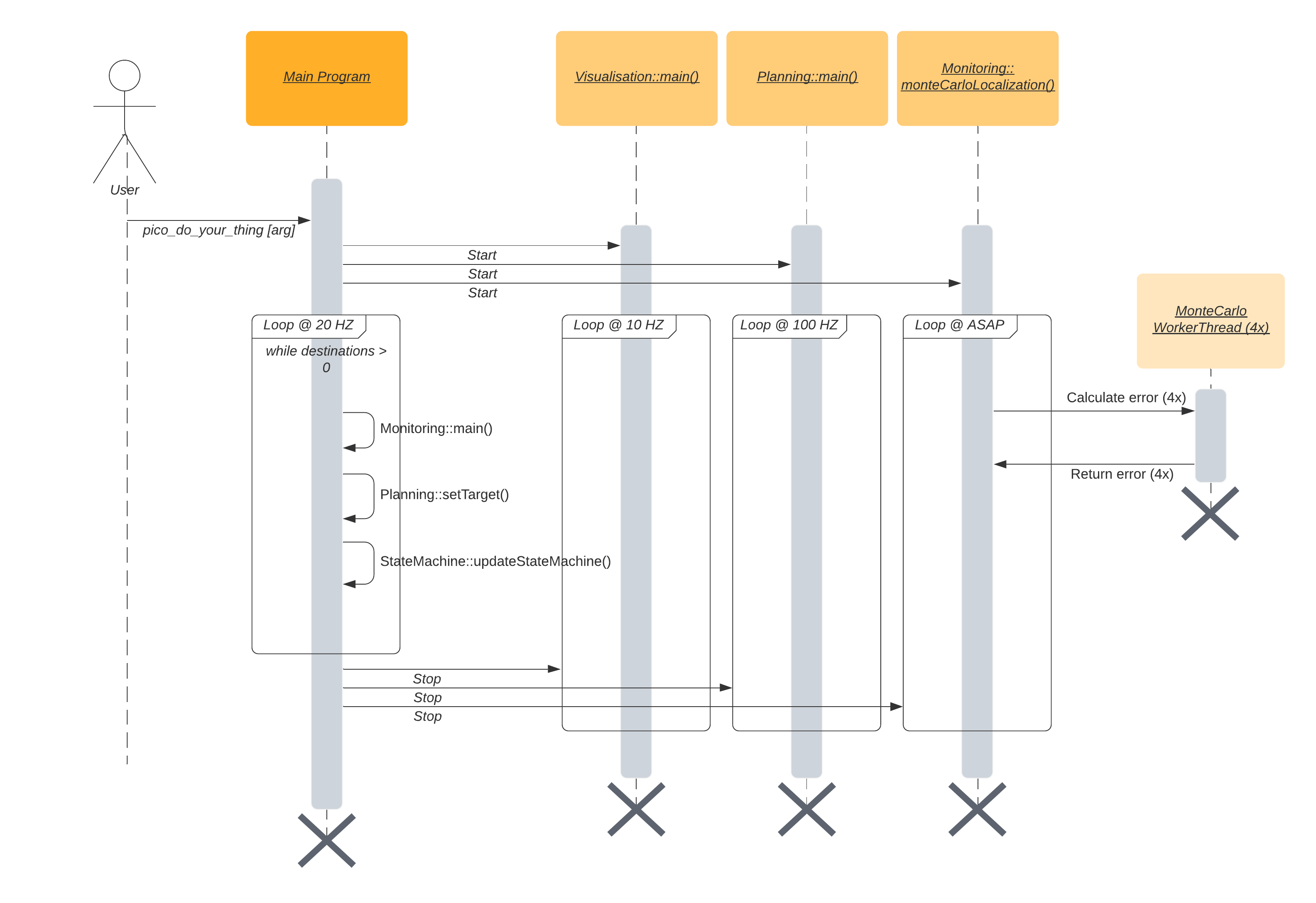
The different components and functions run in an important specified order. The sequence of execution is shown in the sequence diagram below.
The program is started by the argument ‘pico_do_your_thing’. Using this command, the amount of cabinets and the order of the cabinets is specified to the robot. The main loop of the robot keeps on looping until there are no more destinations to be reached. This loop excecutes the MONITORING, PLANNING SET TARGET, and STATEMACHINE code. Three processes run in parralel with this code; the VISIUALISATION, the main planning loop, and the MONTE CARLO LOCALIZATION.
The visualization is run independently from the main code. The visualization is not essential for the main code of the robot, but does give tremendous insights in the behavior of the robot. In order to reduce the computational power required to run the program, the refresh rate of the visualization is reduced compared to the main loop
The main planning loop does not contain the code which determines the target and the path of the robot, but does contain the nessecary control components of the robot. The potential field algorithm, as well as the drive control functions are present in the main planning loop. These functions should be placed in a different loop, but during the testing of the code, this structure ‘snuck in’ to our code, and proved not to be problematic.
The Monte Carlo Localization is also run seperately from the main loop. The main reason for this choice is the very long run time of the localization compared to all other threads. While the goal is to run the localization as soon as possible (ASAP), the realistic runtime approaches 6 seconds per iteration, even when the localization is run on 4 threads.
World model [Koen]
The world model is used as a database. This database is separated into two maps: A global map and a grid map. All gathered data is stored in the world model and then can be used by other processes. Besides the data structures, the world model also has a couple of functions to update the model and extract data from it. The main function is "initGlobalMap", this is the initialization of the global map. Then the function "addWallToGridMap" is used to update the gridmap with all the statics walls. These functions will be described further below. Next to those main functions there are some smaller functions to update or extract odometry data,laser data, robot position and more.
Data structures
The data structures that are shown below are an addition of the UML diagram shown in Components. The main data structure is the Map. This Map contains all the information from the provided JSON file and is used to create both maps. The basic building block of the map is the node. The more complex objects are made by pointing to the nodes.
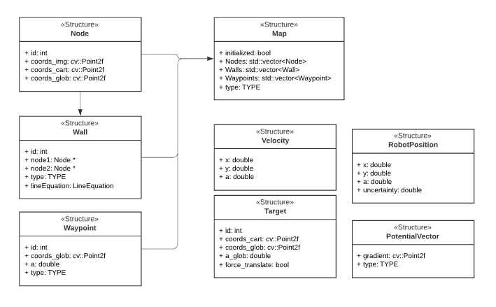
Functions
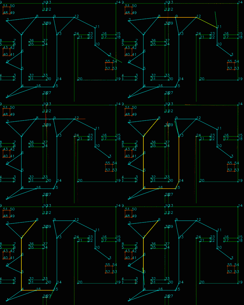
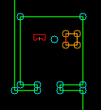
initGlobalMap: This function loads a modified json and turns into into a global map as seen in picture **. Th json file consists of nodes, walls, cabinets and waypoints in front of the cabinets. Every item in this list will be visualized, this is done to make debugging easier. This global map is used as a reference base of the grid map and used to make a clearer visualization.
addWallToGridMap: This function is used to create the basic grid map. It will use the walls that are supplied by the global map to fill in the grid map. This gives a solid base for a initial path planning.
Planning
The planning is made up of two major components: Target determination and path planning. The target determination is done based on the different states Pico can be in. During all states, but the GOTO_NEXT_WAYPOINT, ARRIVED_AT_WAYPOINT, TRANSLATE_TO_WAYPOINT and APPROACHING_CABINET states, the target is set to the current robot position to ensure the robot does not move. During the PLAN_PATH state, the A* algorithm is called to plan a new path to the next destination. During the GOTO_NEXT_WAYPOINT and ARRIVED_AT_WAYPOINT states, the target coordinates are set by the coordinates of the next waypoint on the current path. If the waypoint is reached, it is removed from the current path and the next waypoint is set as the target. During the TRANSLATE_TO_WAYPOINT the target is a predetermined waypoint just in front of a cabinet. When this waypoint is reached the state switches to APPROACHING_CABINET and the target is set such that Pico moves forward slowly.
Path Planning
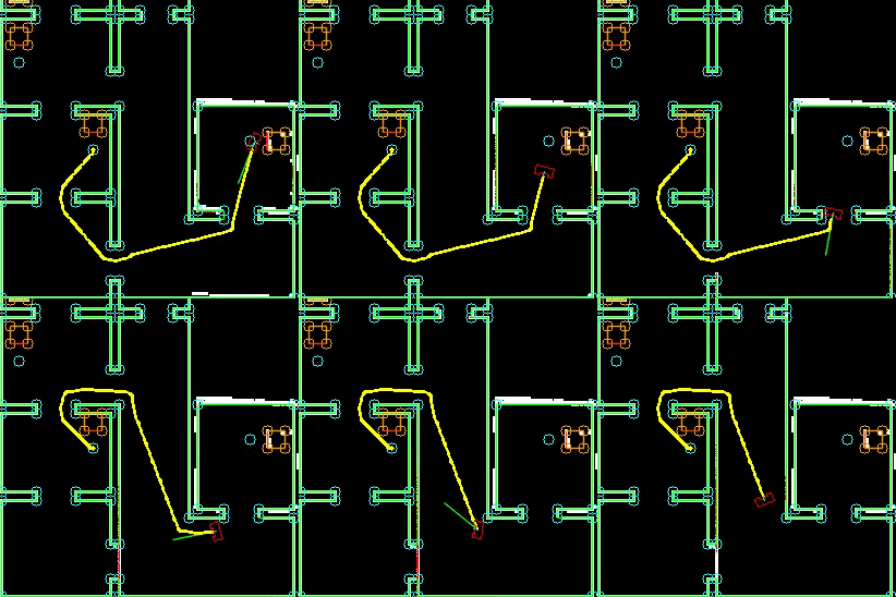
For the path planning the A* algorithm is used. The A* algorithm is an informed search algorithm, meaning that it calculates the path based on weighted graphs or gridmaps. A* determines which of its paths to extend based on the cost of the path and an estimate of the cost required to extend the path all the way to the goal. In mathematical terms, A* selects the path that minimizes:
- [math]\displaystyle{ f(x) }[/math] = [math]\displaystyle{ g }[/math]([math]\displaystyle{ x }[/math]) + [math]\displaystyle{ h }[/math]([math]\displaystyle{ x }[/math])
Where [math]\displaystyle{ x }[/math] is the next node on the path, [math]\displaystyle{ g }[/math]([math]\displaystyle{ x }[/math]) is the cost of the path from the start node to [math]\displaystyle{ x }[/math], and [math]\displaystyle{ h }[/math]([math]\displaystyle{ x }[/math]) is a heuristic function that estimates the cost of the cheapest path from [math]\displaystyle{ x }[/math] to the goal.
The heuristic function is the Euclidian distance between [math]\displaystyle{ x }[/math] and the goal, this means that the heuristic function is admissible. In other words: A* is guaranteed to return the least-cost path from start to goal.
The cost function [math]\displaystyle{ g }[/math]([math]\displaystyle{ x }[/math]) is based on the grid map generated from laser data. If a laser can is reflected at a grid point, the grid point is eventually flagged as blocked. A blocked grid point has a high integer value and a unblocked grid point has a value of zero if it is not close to a blocked grid point. The closer a unblocked grid point is to a blocked grid point, the higher the integer value of the grid point, thus also the higher the cost. To end up with the shortest path, the grid point values are raised by one and multiplied by one if [math]\displaystyle{ x }[/math] is a direct neighbor of the current node and multiplied by √2.
A* has some conditions which determine whether it is possible for a path to be planned. The simplest two are that the starting node and the goal node have to be reachable, meaning that their grid points are not flagged as blocked. The other condition is that there is a free path between the start node and the goal node. This free path in this implementation is a dynamic factor. To ensure that Pico does not collide with static objects, the grid map contains a certain range around blocked grid point where the values of the grid points are higher than zero. For the first iteration of the definition of a free path is that there is a unbroken line of grid points (diagonal counts as well) with a value of zero. This implies that Pico stays well away from all objects. If Pico cannot find a free path after the first iteration, the threshold of accepted grid point values is raised to incorporate the first row of grid points which is effected by a blocked grid point. The threshold keeps decreasing if no path is found until all grid points, except for the blocked grid points, are used by A*. If a path is found, the threshold is reset to its initial value.
Control
The control of Pico is made up of two components: An artificial potential field and a function which determines the different velocities that are fed into Pico's base.
Artificial potential field

The path planning already accounts for a large deal of the obstacle avoidance, but it is not perfect on its own. Furthermore, the path planning is limited to planning a path around static objects. Any dynamic object is not picked accounted for in the gridmap used for the path planning. To solve these issues it is opted to use an artificial potential field, APF in short. The philosophy of the artificial potential field approach can be described as follows:
The manipulator moves in a field of forces. The position to be reached is an attractive pole for the end effector and obstacles are repulsive surfaces for the manipulator parts.
In this case, the position to be reached is the next path point. Since the APF is only used as a last resort for obstacle avoidance, we do not want the full effect of it at all times. To this end, the effect of the APF will only be exploited when Pico sees an obstacle within a certain range. At this particular range, the repulsive potential vector starts to increase from zero.
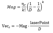
The repulsive potential vector is created from the live laser data Pico gathers at all times. If a laser beam has a range between the minimal range of the LRF and a maximum free distance around Pico, a vector is calculated in the following manner:
Here [math]\displaystyle{ \eta }[/math][math]\displaystyle{ r }[/math] is a constant to scale the magnitude. [math]\displaystyle{ k }[/math] is a value to change the slope of the magnitude, higher values for [math]\displaystyle{ k }[/math] give a steeper slope. [math]\displaystyle{ D }[/math] is the distance between the robot and the laser point, or effectively the range of the laser beam. [math]\displaystyle{ \Delta }[/math] is the safe distance around Pico, for values of [math]\displaystyle{ D }[/math] higher than [math]\displaystyle{ \Delta }[/math] nothing will happen. The other way around the magnitude will increase. Finally laserPoint is the point in the local robot coordinate frame where the laser beam is reflected by an object.
Every laser beam results in an Vecr. To final repulsive vector used in the actual control of the robot is the summation of all Vecr. In this way vectors from adjacent sides are able to cancel each other.
For the final implementation of the APF only the repulsive vector is used. The vector to the next path point is taken as the attractive vector. Only when there is a repulsive vector with a magnitude greater than zero, so when there is an object within a distance [math]\displaystyle{ \Delta }[/math] from Pico, the repulsive vector is added to the attractive vector to act as a collision avoidance measure. To ensure that Pico will never run into any object, the APF is updated at an increases rate of 100 Hz. It is chosen to do this at a higher rate, since lower rates like 20 Hz would induce a oscillation if Pico was blocked by objects on two different sides, eventually leading to a collision.
A downside of the APF approach is the existence of local minima in which one could get stuck. For this implementation the local minimum does not really cause any problems, since the solutions are accounted for by other parts of the code. For instance, when a new object is detected on the current path of Pico, a new path is calculated. If Pico does find itself in a narrow situation, the path planning is optimized to find the best path possible within the boundaries provided by Pico.
Velocity determination
The velocity and direction of Pico depends on the location of the next target with respect to the location and orientation of Pico and on the repulsive force of the APF. The location of the next target and the repulsive vector are given as vectors in the local Cartesian coordinate frame of the robot. If there is a repulsive force generated by the APF, the target vector and the repulsive vector are summed. This resulting vector is the basis of the lateral and longitudinal velocity of Pico. The angular velocity is solely determined by the angle of the target vector.
The velocity which is send to the Pico base is determined by an based on a few conditions. In the "APPROACH_CABINET" state Pico is forced to translate, whilst in the "ORIENT_TO_CABINET" state Pico is forced to rotate. In the other states Pico will purely rotate if the angle [math]\displaystyle{ \theta }[/math] between the robot and the target is too large, purely translate in the longitudinal direction if [math]\displaystyle{ \theta }[/math] is small enough, and have a combined movement of rotating and translating in both directions if [math]\displaystyle{ \theta }[/math] is in between the two boundaries. If there is a repulsion force, the minimum angle is ignored for the combined movement.
Monitoring [Friso]
The monitoring component has the job of tracking and updating the robot's current position and it's surroundings. This class consists of two main parts: mapping of the robot's actual surroundings (incl. static clutter) and determining the exact position of the robot within the given global map using laser data. Mapping the surroundings is done using 'Occupancy Grid Mapping'[2] and localization using laser data has been accomplished by implementing so called Monte Carlo localization.
Occupancy grid mapping (static clutter detection) [Friso]
To be able to create correct and efficient paths through the hospital, the robot has to be in possession of a complete and actual map of it's surroundings. This is done using Occupancy Grid Mapping. In this technique, a gridmap is drawn over the (given) global map, with each grid-square containing a single value indicating whether or not that grid-square is occupied (traversable) or not.
Populating the gridmap
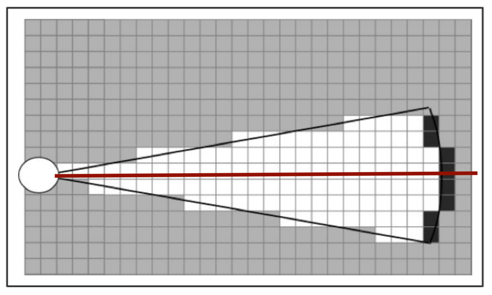
Populating the gridmap is done once at program startup and then updated every main-program cycle. During initialization and interpretation of the given .json-map, the each grid-square being crossed by a wall or cabinet is assigned a value of GRID_WALL_VALUE (100.0).
During the execution of the program, the grid-squares' values are updated using the currently seen laserpoints. For each laserpoint, the corresponding grid-square in which it's located is determined and this grid-square's value is increased by GRID_LASER_BLOCKED_VALUE (0.5). Even more, the grid-squares positioned in between the robot's current location and the laserpoint's position are determined as being empty and have their values subtracted by GRID_LASER_FREE_VALUE (0.5). This uses the fact the robot wouldn't have been able to see an object if the grid-squares in between the object and the robot are not empty. Determination of which grid-squares are in between the robot and the laserpoint is done using a Bresenham algorithm implementation from tech-algorithm.com.
The ability to 'open up' grid-squares after they have been determined as being occupied, either by the initializing sequence or object detection, is crucial in creating a robust system being able to handle the imperfect world. E.g. dynamic clutter, doors or walls being in a slightly different position w.r.t. the given .json-map, being able to fix the gridmap after populating it with incorrect data due to an error in localization, etc.

Interpreting the grid-map
Since the gridmap consists of a collection of grid-squares, all possessing a value, this value has to be translated to a portion of the map being occupied or free. This is done by checking if the grid-square's value is above GRID_LASER_FREE_VALUE (0.5), if so, the grid-square should be interpreted as being occupied. This is done e.g. in the visualizer and in the planning of the path of the robot.
Preparing the gridmap for path planning use
The path planning algorithm (A*) does not use the 'raw' gridmap as described above. Instead, it uses a processed copy (gridMapRanges) which adds a region of obstruction around the detected objects with values tapering off the further away from this object. It normalizes all grid-square values to the range [0, 255]. These values are used by A* in a way it'll prefer staying away from objects but still being able to do come close if absolutely necessary. The exact workings of A* and it's using of these grid-square values can be seen at the 'Planning & Control' section on this page.
For each grid-square which has been identified as occupied (grid-square value > GRID_LASER_FREE_VALUE), the grid-squares present in a circle of GRIDMAP_RESOLUTION * 6 (0.5 * 6) around the occupied grid-square are affected and have a value between 0 and 255 assigned to them. This is done using the following formula, in which [math]\displaystyle{ x }[/math] is the distance of the grid-squarew.r.t. the occupied grid-square diveded by GRIDMAP_RESOLUTION.
Monte Carlo localization [Friso]
Monte Carlo localization is used in order to determine the position of the robot within the map. Due to the initial position of the robot being roughly known and the ability to track the (rough) position of the robot using odometry data, this method is a relatively easy way to get an exact position whilst being relatively robust.
In this approach, a group of different robot positions is generated and a estimation is made on how well the current observations (laser points) fit each possible position. The one most likely to be the correct position is then chosen. The different steps of this process are explained below.
Generation of Monte Carlo positions
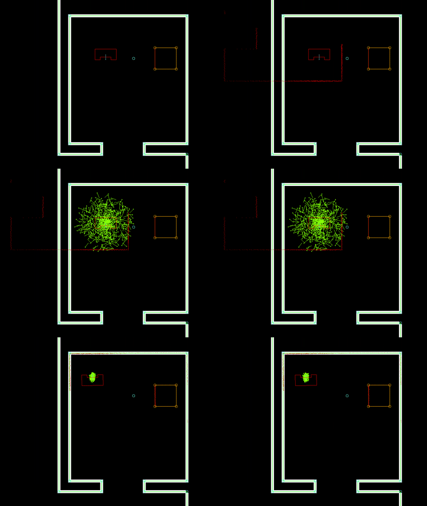
Possible new positions of the robot (Monte Carlo positions) consist of a position (x- and y- coordinates) and an orientation (angle). These positions are generated in a radius around the current robot position. The orientation of these positions are taken from a normal distribution around the current robot position's orientation. The exact way of calculating these values is related to the 'uncertainty' value of the current robot position. The higher this value, the greater the radius of the circle in which the positions are generated, the standard deviation of the normal distribution used and the amount of positions generated. This has two reasons:
- If uncertainty is low, the amount of Monte Carlo positions generated can be minimized to reduce computational intensity and, in turn, runtime
- If uncertainty is low, the same amount of positions can be distributed along a smaller area and orientation range. This can improve accuracy of the found position
This uncertainty value gets increases over time and is reset once a new position is determined using Monte Carlo. The new value is related to how much the robot has moved since the previous time the position has been determined using Monte Carlo. This uncertainty value is used in the generation of the Monte Carlo positions which are going to be checked.
Selecting the best Monte Carlo position
For each position, the likelihood of the position being the actual robot position has to be determined. This is done by calculating an 'error' value for each position. This is done by going through the currently seen laserpoints (with a position w.r.t. the robot), placing these points within the global map using the Monte Carlo position and determining the distance to the closest wall or cabinet. These distances are summed for all laserpoints and together make up the error value. The position with the lowest error value (in effect, the position in which the seen laserpoints line up with the given .json-map the best) is selected as a new robot position candidate. A last check is done to verify the found position is within reason (it's not unreasonably far away from the current position) and if so, it's set as the new robot position and the new position uncertainty is set.
V
E
R
T
I
C
A
L
S
P
A
C
E
Perception [Koen]
The perception module reads out the laser and odometry sensor data and writes it to the world model. Because these are different sensors, the frequency at which the data is updated is different. This resulted in very clunky behavior of the systems that use this data. To reduce this, the data is paired based on their timestamp.
Statemachine [AJ]
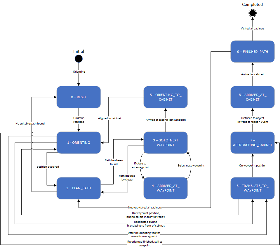
The state machine designed for the hospital challenge is described in this paragraph.
RESET
The first state is the RESET state, this state will be executed when the program is initially started and will reset the grid map. This state will also be executed when the path planning is not able to find a suitable path to the current target. By resetting the grid map all previous detected clutter will be erased, when the gridmap is resetted the ORIENTING state will be executed.
ORIENTING
The localization of the robot within the world model will be done in the orienting state based on the Monte Carlo algorithm. When the localization is successfully executed and the position uncertainty is low enough, then the state machine will continue based on these three statements:
- If the last state was equal to ORIENTING_TO_CABINET, and the distance from the current robot position and the cabinet is smaller then the MIN_WAYPOINT_DISTANCE(0.15), then the state machine will continue to APPROACHING_CABINET. This means that position of the position of the detected cabinet is shifted with the location of the JSON cabinet position, so a reorientation is acquired to align with the JSON map.
- If the last state is also equal to ORIENTING_TO_CABINET, but the distance is larger then the MIN_WAYPOINT_DISTANCE(0.15), then then the state machine will continue to TRANSLATE_TO_WAYPOINT. This means that a reorientation is required but the cabinet waypoint is to far away to approach the cabinet based on the laser data, so instead the robot will just translate to the cabinet waypoint.
- If the last state is equal to TRANSLATE_TO_WAYPOINT, then after the reorientation the state machine will return to TRANSLATE_TO_WAYPOINT. In this case the a reorientation is acquired during the translating process, so after the reorientation the state machine will directly return to the TRANSLATE_TO_WAYPOINT state.
- If these three conditions are not fulfilled than the PLAN_PATH state will be executed, this means that the program is started from its initial condition or the clutter is cleared by the RESET state.
PLAN_PATH
In the PLAN_PATH state the actual path planning algorithm is exacted, when the the program is started from the initial condition, the optimal path is generated to the target waypoint based on the A-star algorithm. When the robot path is determined, the state machine will continue to the GOTO_NEXT_WAYPOINT state, if the GOTO_NEXT_WAYPOINT state is not able to reach the target waypoint or the A-star algorithm is unable to plan a suitable path, then the PLAN_PATH state will call the RESET state to clear the grid map. If the PLAN_PATH state is called by FINISHED_PATH which means the path to the next cabinet must be generated, the plan path cycle starts again.
GOTO_NEXT_WAYPOINT
The GOTO_NEXT_WAYPOINT state makes sure that the robot follows the generated set of waypoints towards the cabinet, if the current waypoint is reached the state machine switches to the ARRIVED_AT_WAYPOINT. This process will repeat till the last waypoint of the planned path is set as current target, when this is the case then the ORIENT_TO_CABINET will be executed. If the robot is unable to reach its target waypoint duo to clutter blocking its path, then the PLAN_PATH state is called.
ARRIVED_AT_WAYPOINT
At this stage there will be checked if the target waypoint is within the MIN_WAYPOINT_DISTANCE(0.15), if this is the case then the state machine will switch back to GOTO_NEXT_WAYPOINT.
ORIENTING_TO_CABINET
When the robot is driving to the last waypoint of the planned path, the robot will rotate till it is aligned parallel with the cabinet. Afterward the ORIENTING state is called to reorientate in front of the cabinet.
TRANSLATE_TO_WAYPOINT
when the robot is reorientated and the distance to the cabinet waypoint is larger then the MIN_WAYPOINT_DISTANCE(0.15), then the robot will translate to this waypoint. In this state is the robot also allowed to drive backward to prevent that the robot has to rotate again to align with the cabinet. If the robot is not able to reach the cabinet waypoint due to a reoreintation error, the ORIENTING state will be called and a second attempt to translate to the waypoint will be executed. When the robot reaches this waypoint the state machine will execute the APPROACHING_CABINET cabinet state.
APPROACHING_CABINET
In this state the robot is positioned in front of the cabinet, and will drive based on the laser data towards the cabinet, until the robot is positioned at a distance of 30 cm to the cabinet. If this is the case the ARRIVED_AT_CABINET will be called.
ARRIVED_AT_CABINET
With the robot positioned correctly in front of the cabinet, there will be communicated with IO speak "I have arrived at cabinet X" and the state state machine will continue to FINISHED_PATH.
FINISHED_PATH
when the robot has successfully reached the target cabinet there will be checked if this is the final cabinet, when this is the case then the COMPLETED state will be called otherwise the state machine will continue to PLAN_PATH and the cycle will be repeated.
COMPLETED
This state is reached when all cabinets have been visited. The robot shuts down when this state is reached.
User interface [Koen]

The main function of the interface is to show the current state of the robot in the world and what it will do next. This information can be used to more efficiently debug the code. The interface is created by the visualization scrip. This component uses the information from the world model to visualize the map. The information that is visualized can be adapted by activating or deactivating various parts, this can be done either in the code or on the visualized map itself. The interface has also the option to turn on manual control, this way it is easy to test specific positions of the robot.
The visualization also shows all the threads which are running, and their respective runtimes. The set runtime is given, as well as the actual runtime. This proved to be very helpfull in identifying computationally intensive tasks. If a thread would run for much longer than its originally set run time, some changes had to be made.
e
x
t
r
a
v
e
r
t
i
c
a
l
s
p
a
c
Testing [Sjors & AJ]
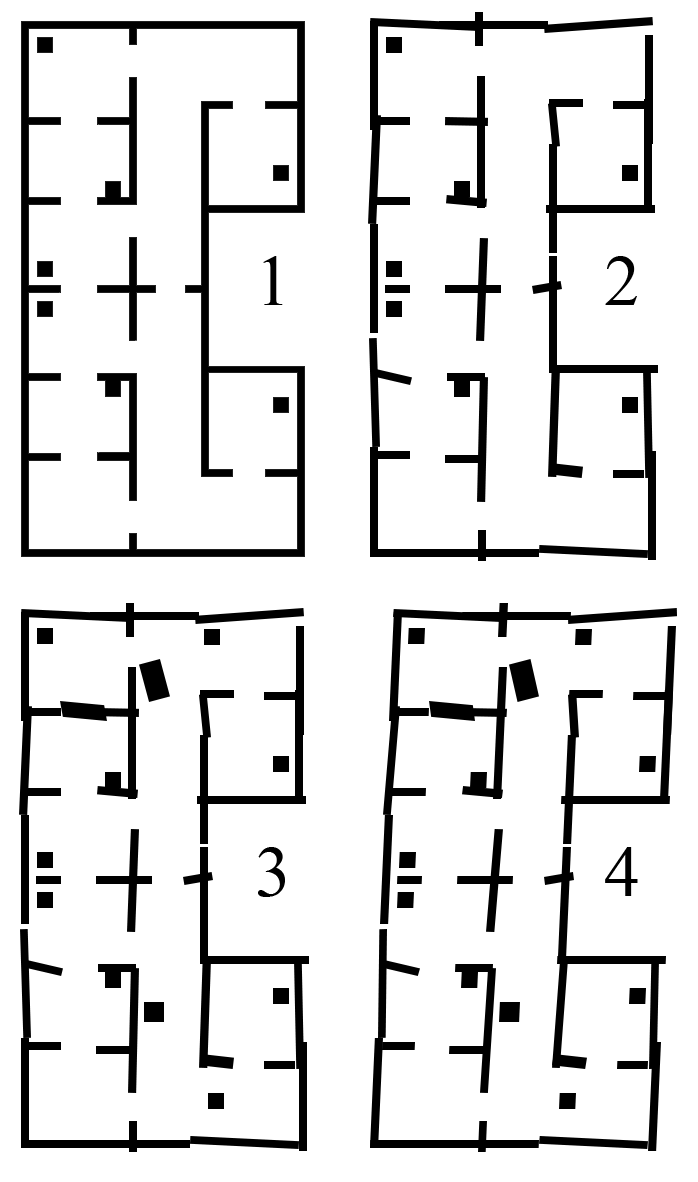
The robot must the thoroughly tested before the final challenge. The robustness of all components must be tested and changed if needed in order to be sure that the robot can handle unexpected situations during the hospital challenge. Three main points have been tested in order to assure robustness: Imperfect maps, clutter objects and path planning obstacles.
Imperfect maps
Different versions of the hospital map were used during testing. The difficulty of the maps was increased over time, in order to tackle different aspects seperately. The .json file, which gives a perfect map of the hospital lay-out is given, which was used during the first stages of testing. It must be noted that this 'perfect' version of the map is not sufficient for testing purposes. The imperfect maps have been created in order to test the robustness of the robot. The added imperfections include holes in the walls, offset walls and cabinets, and skewed maps. The different stages of the imperfect maps are shown in the Figure below.
The first custom test map, and thus the second testing map, contains multiple gaps between walls, as well as misplaced wall segments. This simulates the real enviromnment, where different imperfections are present.
The third testing map includes extra static clutter. The static clutter is placed at key positions where the robot normally would drive in order to complete its tasks. The path planning of the robot, as well as the way it deals with extra clutter objects is tested using this map.
The fourth map includes a large skew angle. The bottom part of the map stays relatively close the original map, while the top of the map has a big offset. The overall error regadring misplaced segments therefore increases vertically. This allowed the use of 1 map for an increasing amount of error. The robot was first tested at the bottom half of the map. When it was concluded that the robot could handle the small errors at the bottom of the map, the robot was tested at the top half of the map, which proved to be more difficult.
Results
Eventhough the walls were not perfectly aligned with the .json map, the robot had little problems navigating through the map. The grid map in combination with the potential field ensured that the robot would not run into walls, even when walls were completely in the wrong place.
An exceptional case in which the robot would fail to navigate through the hospital is when the walls are offset so much that the combination of the seen walls and the predetermined locations of the walls block the entire path. This unique case would require a huge difference between the .json map and the simulation map. It is therefore assumed that this would not be the case during the final challenge.
The localization in skewed maps also proved to be difficult. If the initialization and localization at the start fail, and have a rotational offset, the robot got lost with no way of getting back on track. This problem was solved by changing the conditions and the thresholds of the first initialization. Once the position was well established the robot was allowed to continue.
The static avoidance of the robot is visualized in the animation shown below. The two small blocks near the beginnen of the trajectory are avoided. The big clutter object further down the path is immediately avoided once the robot has seen the object. The path is changed accordingly.
Path planning
A different path planning strategy was used in the early stages of the project. This strategy used manually set waypoints throughout the map, and Dijkstra's algorithm to navigate through these waypoints. The links between the waypoints can be made inactive if an obstruction on the path of the robot is observed. Though this strategy was promising, it was eventually discarded in favor of the gridmap and A* approach. This choice was made based upon robustness. A lot of manual waypoints must be placed in order to ensure that the robot can drive through the hospital with all kinds of different clutter configurations. This way of 'hard coding' the path also seemed like a rather messy solution.
This animation shows how Dijkstra's algorithm was implemented. This particular case has an added obstruction between waypoint 8 and 9. The robot wants to go through this closed door, but is stopped by the potential field. After some time, the robot realizes that this link is invalid, and calculates a new path around the obstacle.
Clutter
The addition of static clutter was handeled very well by the robot. The gridmap proved to be an excellent tool for this, since every small piece of obstruction can now be tracked and taken into account when planning a path. The dynamic clutter was added in the same fashion, but the removal of previously occupied grid spaces was not finely tuned. This would result in a large smear of occupied grid spaces caused by a dynamic object. After fine tuning the parameters, the dynamic clutter was robustly taken care of by the robot
Evaluation
Evaluation of design process
- switching strategies quite often, and maybe too late. Next time think things through a little more before you commit to something.
Evaluation of challenge
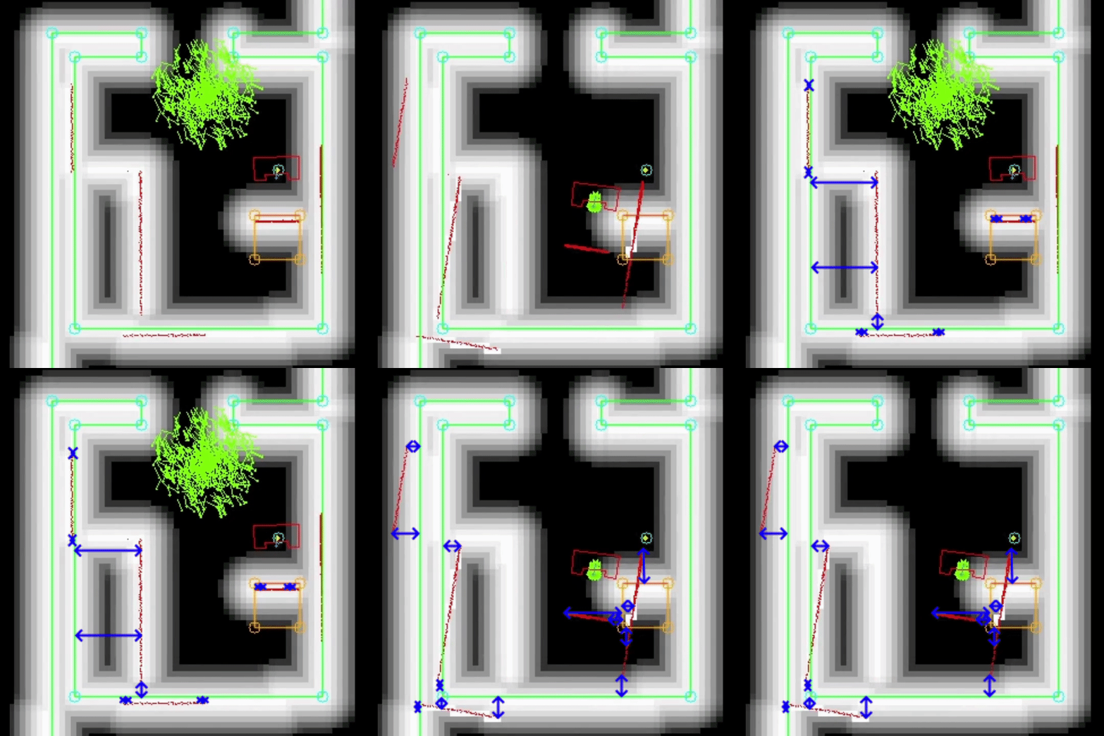
In this video, a run of the final program of the final map can be seen. Since no video of the actual (live) challenge is available, this run has been recreated at a later time. The behavior is exactly the same however. One thing has been changed in the visualization w.r.t. the program ran during the challenge. Instead of only showing the grid with the actual clutter, the ranges which are placed around this clutter and used by the path planning algorithm are shown aswell. This way, it's easier seen when/why certain behavior happens. The enabling of this visualization was not done during the live challenge, due to the extra resources this requires. The visual hiccups which seem to appear in the video (drop in framerate) where not visible during actual recording and are most probably an artifact of the recording software used.
Although a lot of things went well, such as avoiding collisions and immediately determining a new path after detection of clutter, the program encountered problems at the second cabinet (cabinet nr. six). This exact failure occurs at each try of this map at cabinet six. This has to do with the implementation of the used Monte Carlo localization algorithm.
Why did it fail?
Arrival at the cabinet is determined by it's global position w.r.t. the waypoint in front of the cabinet. Due to position errors which can occur during travel, a 're-orienting' state has been added before actually approaching the cabinet it should be in front of. In this state, the localization algorithm is ran three times and the regular limits w.r.t. maximum allowable 'jump' in position are removed. In this room however, this results in problems. In the shown video, it's visible what the situation is when arriving at the cabinet, and the new position which the robot thinks is the correct one. A human can clearly see the initial position is off by a few centimeters, but more or less correct. The new position however, is completely tilted and wrong. The algorithm disagrees however. Also shown in this video, is the way the error of the different positions is calculated. This error is the sum of all distances between a subset of the laserpoints and it's closest wall or cabinet. This indicated by the blue arrows. Now, it's easily seen why the algorithm chooses this position: the sum off all distances is lower, even though a lot of individual distances are actually increased.
What can be improved?
Of course, multiple approaches can be taken in solving this problem. E.g. instead of re-orienting the complete (global) position of the robot, the choice could be made to switch to a local navigation method. After arriving at the approximate position in front of the cabinet, the geometry of the cabinet could be recognized and target determination be done using the exact position of this recognized geometry. In this case however, it's clear the Monte Carlo algorithm can use some improvement. It's not only quite slow (as indicated earlier in this document), it also selects positions easily identified as incorrect by a human observer. Below a list of steps which can be taken to improve the performance of the Monte Carlo localization:
- Instead of looking at all geometry in the map, only check distances of the laserpoints w.r.t. geometry the robot is expected to see from it's current (approximate) location. This not only removes the option of using the distance between a laserpoint and the back-side of a wall, but (if implemented efficiently) could also reduce computational costs by reducing the amount of maximum distance calculations required.
- A preference for positions in which most points have a negligible distance to a wall or cabinet (e.g. 5 cm) instead of only looking at the average distance of all laserpoints w.r.t. a wall or cabinet.
References
- ↑ Bruyninckx, Herman. "The design of a RobMoSys' Share-all component", KU Leuven - TU Eindhoven, 2020. Bruyninckx
- ↑ [[Cyrill Stachniss, "Robot Mapping - Grid Maps", Uni Freiburg]] Autonomous Intelligent Systems
