Embedded Motion Control 2014 Group 11

Go back to the main page.

Group Members

Name:	Student id:	Email:
Groupmembers (email all)
Martijn Goorden	0739273	m.a.goorden@student.tue.nl
Tim Hazelaar	0747409	t.a.hazelaar@student.tue.nl
Stefan Heijmans	0738205	s.h.j.heijmans@student.tue.nl
Laurens Martens	0749215	l.p.martens@student.tue.nl
Robin de Rozario	0746242	r.d.rozario@student.tue.nl
Yuri Steinbuch	0752627	y.f.steinbuch@student.tue.nl
Tutor
Ramon Wijnands	n/a	r.w.j.wijnands@tue.nl

Time survey

The time survey of this group will be hosted on a Google drive. Therefore, all group members can easily add information and anyone can see the up-to-date information. The document can be accesed by clicking this link: time survey group 11

Planning

Week 1 (28/4 - 4/5)

Finish the tutorials, including

• installing Ubuntu,
• installing ROS
• installing SVN
• get known with C++
• get known with ROS

Week 2 (5/5 - 11/5)

Finish the tutorials (before 8/5)

• Setting up an IDE
• Setting up the PICO simulator

Work out subproblems for the corridor competition (before 12/5)

Comment on Gazebo Tutorial

When initializing Gazebo, one should run the gzserver comment, however, this can result in a malfunctioning program, i.e. you will get the following message: Segmentation fault (core dumped). The solution for this is to run Gazebo in debugging mode (gdb):

1. Open a terminal (ctrl-alt-t)
2. Run:

   gdb /usr/bin/gzserver

   when (gbd) is shown, type run and <enter>
3. Open another terminal (ctrl-alt-t)
4. Run:

   gdb /usr/bin/gzclient

   when (gbd) is shown, type run and <enter>

Comment on running Rviz

Simular to the Gazebo tutorial, the command rosrun pico_visualization rviz can also result in an error: Segmentation fault (core dumped). Hereto, the solution is to run Rviz in debugging mode:

1. Open a terminal (ctrl-alt-t)
2. Run:

   gdb /opt/ros/groovy/lib/rviz/rviz

   when (gbd) is shown, type run and <enter>

Moreover, in order for the camera to work properly, in the Displays view on the left change the Fixed Frame.

Week 3 (12/5 - 18/5)

Finish the corridor competition program.

Week 4 (19/5 - 25/5)

Update the wiki page with current software design. Optimize current software nodes. Determine workload for implementing SLAM and a global controller.

Week 5 (26/5 - 1/6)

A launch file is created to run the multiple nodes at once. Currently, it runs the following nodes:

• Target
• Path_planning
• Drive

To apply the launch file, execute the following steps

1. Start the simulation up to and including

   roslaunch pico_gazebo pico.launch

2. Open a new terminal (ctrl-alt-t)
3. Run:

   roslaunch Maze_competition pico_maze.launch 

Maze competition

The goal of this course is to implement a software system such that the provide robot, called PICO, is able to exit a maze autonomously. Embedded software techniques provided in the lectures and literature need to be implemented in C++. The ROS concept is used as a software architectural backbone.

The PICO robot has three sources of sensor information available to percieve the environment. First a laser provides data about relative distances to nearby objects (with a maximum distance of 30 meter). Secondly, images can be used to search for visual clues. Finally, odometry data is available to determine the absolute position of the PICO.

PICO can be actuated by sending velocity commands to the base controller. The PICO is equipped with a holonomic base (omni-wheels), which provides the freedom to move in every desired direction at any moment in time.

The assignment is successfully accomplished if the PICO exits the maze without colliding with the walls of the maze.

Software design

The current ROS node structure is shown in the figure below.

The nodes /GazeboRosLaser_node and /pico/pico_state_publisher are predefined ROS nodes. Currently, four extra ROS nodes are added:

1. /Target: This node determines the target where the PICO has to drive to. The node has as input the laser data and velocity commands, and produces a point expressed in relative coordinates. If multiple interesting targets are found, it returns the most left or most right target (which can be chosen before starting this node).
2. /Potential_field_direction: From a given target, it produces a path to that target. It generates this path by using potential fields, where walls have high potentials and the target a low potential. It returns a direction where the PICO has to go at that moment in time.
3. /Drive: It translates the received direction into a translation and rotation speed. This node is able to change the direction if it notice that the PICO is to close to a wall.
4. /slam_gmapping: This node produces from the laser and odometry data a map of the maze. This allows to know the absolute position of the PICO in the maze. Therefore, targets can be memorized to, for example, prevent looping in the maze.

The next table summarize the message types for each used topic.

Topic name:	Message type:
/pico/laser	LaserScan
/pico/target	Point
/pico/direction	Point
/pico/cmd_vel	Twist
/tr	tfMessage
/map_metadata	MapMetaData
/map	OccupancyGrid

In the following sections, the algorithm used in these nodes will be explained in more detail.

Corridor detection system

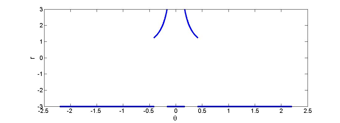
First a horizon R is being set. Every value r(i) > R is being replaced by r(i) = -R. This can be seen in the figure below where R=3.

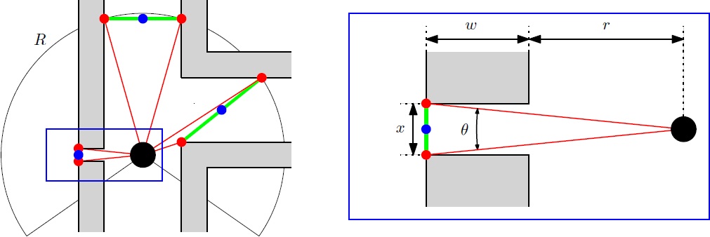
Then the change in the radii are evaluated: dr = r(i+1) - r(i). When dr>R then r(i+1) is saved, when dr<-R then r(i) is saved. A set-point can be set in between the two corridor points. However there are 4 points in this situation (see figure left below), the two central represent the corridor. If there are any outer points, they can be removed from the set (figure center below), this results in at least one pair of 2 corridor points (figure right below shows the possibility of multiple corridor point pairs). Each blue dot is the average in x and y value of a pair of red dots.

However, a small gap can be detected (figure below left). In order to ignore such a gap, the angle difference of the points of a pair are compared with a threshold value. This threshold value is calculated for the worst case scenario: [math]\displaystyle{ \theta=0.1 }[/math] rad when closest to the wall [math]\displaystyle{ r=0.25 }[/math] m, a gap of [math]\displaystyle{ x=4.5 }[/math] cm, the wall thickness [math]\displaystyle{ w=0.2 }[/math] m (see figure below right).

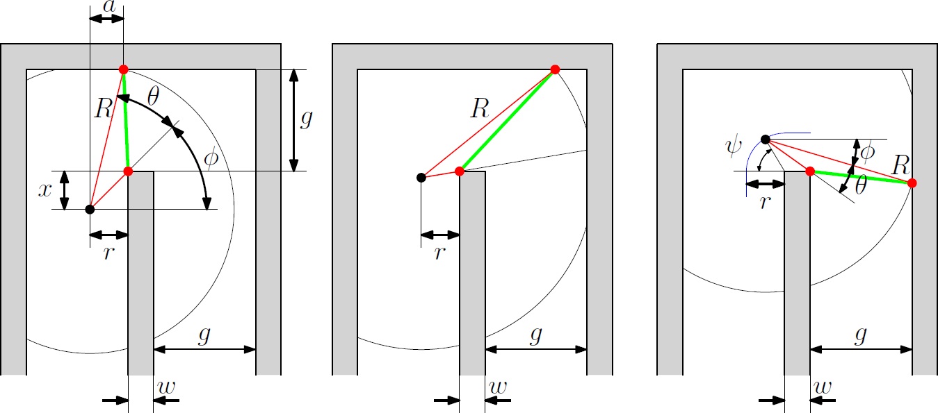
Figure below shows the worst case scenario, a U-turn. The left figure describes the radius R as a function of distance x which has a minimum of [math]\displaystyle{ R=1.148 }[/math] m it is important that the angle should always be larger than the derived [math]\displaystyle{ \theta=0.1 }[/math]. The center figure shows that [math]\displaystyle{ R\lt r+w+g=1.05 }[/math] m in order to maintain the red dot at the center wall up to [math]\displaystyle{ x=0 }[/math] m. The right figure shows what happens beyond the point [math]\displaystyle{ x=0 }[/math] m. In this situation the maximum value for the radius is the smallest one of the three: [math]\displaystyle{ R\lt 1.034 }[/math]. All the values are calculated with [math]\displaystyle{ r=0.25 }[/math] m, [math]\displaystyle{ w=0.2 }[/math] m, [math]\displaystyle{ g=0.6 }[/math] m.

What can be concluded is that the radius should be chosen at 1 m. This causes a problem when entering a crossroad with a road width of [math]\displaystyle{ g=1.5 }[/math] m, then pico can't see the three corridors. Therefore a second radius is added of [math]\displaystyle{ R_o=1.7 }[/math] m.

With the two radii, two sets of corridor points are made. The center of the corridor will be taken as target. It is determined when

• the center of the corridor detected by the small radius is inside 180 degrees vision.
• the corridor pair doesn't represent a dead end.[math]\displaystyle{ {}^* }[/math]
• as said the angle of the pair is larger than [math]\displaystyle{ \theta=0.1 }[/math].
• the gap is large enough for pico to drive through.

When there is no point detected, pico will stay at its current position. When there are one or more points detected, pico will follow the one with the largest or smallest angle (depending on left or right oriented pico)

[math]\displaystyle{ {}^* }[/math] this holds if there is a step in the radius (larger than 40 cm) in between the corridor pair.

Path Planning Pico: Potential Field Approach

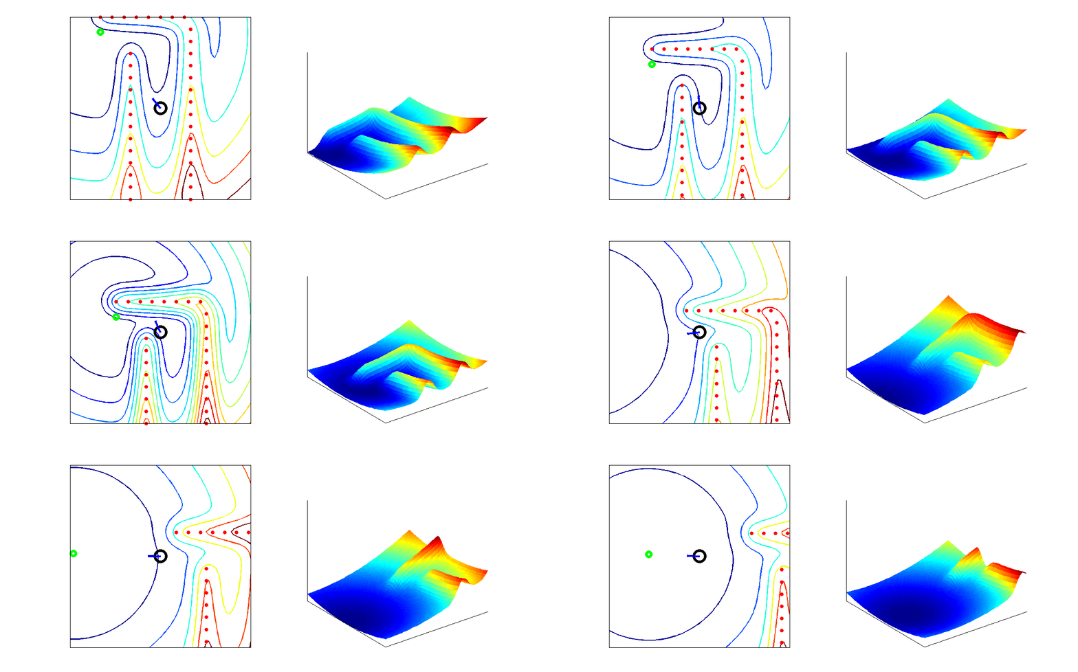
From the higher level control node "Target", Pico will receive a desired local destination. In order to reach this destination in a smooth fashion, a particular path planning method will be employed. This method is based on artificial potential fields. The key idea is that the local target (destination point in 2D space) will be the point with the lowest potential. Everywhere around this target, the potential will be strictly increasing, such that the target is the global unique minimum. Any objects as detected by Pico will result in a locally large potential. The path planning can now be based on any gradient descent algorithm as are often used in optimization problems. Because of the ease of implementation, the first order "steepest descend" method will be used (this avoids having to approximate the Hessian matrix locally. The Newton method may be implemented in the future as it also takes curvature information into account which may improve the overall performance). In the gif below, the main concept is illustrated.

Here, Pico is the represented by the black circle and the smaller red circle is the target. The potential field generated by the target is simply the euclidean distance squared, i.e,

[math]\displaystyle{ P_{target} = (x_{target} - x_{pico})^2 + (y_{target} - y_{pico})^2 }[/math].

The black spots represent the laser measurement data (note that the gif does not give a very realisitic representation of the true measurements). Each measurement point provides a 2D Gaussian contribution to the total potential field, i.e.

[math]\displaystyle{ P_{objects} = \sum_{i = 1}^{1081} exp\left( \frac{-(x_{object_i}-x_{pico})^2-(y_{object_i}-y_{pico})^2}{\sigma^2} \right) }[/math],

where [math]\displaystyle{ \sigma }[/math] is a skewness parameters. The total potential field now becomes,

[math]\displaystyle{ P_{total} = \alpha_1 P_{target} + \alpha_2 P_{objects} }[/math],

where [math]\displaystyle{ \alpha_1 }[/math] and [math]\displaystyle{ \alpha_1 }[/math] are additional tuning parameters. The steepest descent direction is numerically approximated (this could also be done analytically) by constructing a local grid around Pico and computing the central first order difference in both the x- and y-directions,

[math]\displaystyle{ \vec{\nabla} P_{total} \approx \frac{P(\Delta x, 0) - P(-\Delta x, 0)}{2 \Delta x} \vec{e}_x + \frac{P(0, \Delta y) - P(0, -\Delta y)}{2 \Delta y} \vec{e}_y }[/math].

The direction in which Pico should move is now given by,

[math]\displaystyle{  \vec{D} = \frac{\vec{\nabla} P_{total}}{\|\vec{\nabla} P_{total}\|}  }[/math].

This direction will be send to the "Drive" node which computes the appropriate velocities based on this direction.

Driving the Pico

The Pico needs to drive towards the first destination point of the resulting path planning. There are various ways to achieve this by using its two independ velocity componements, namely the translational speed [math]\displaystyle{ \dot{x} }[/math] and its rotational speed [math]\displaystyle{ \dot{\theta} }[/math]. One could for instance first rotate the Pico in the right direction, to subsequently just drive forwards until the destination is reached. However, this can be a time consuming task as the Pico has to stop each time a correction on the direction has to be made. Moreover, when a corner needs to be taken, mutlitple waypoints are necessary to guid the Pico. Therefore, an alternative algorithm is developed, which can react more quickly on directional changes and steers the Pico as fast as possible towards its destination. The concept of this algorithm is shown in the figure to the left.

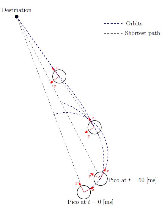
Here an extreem situation is sketched, to fully illustrated the functioning of the method. In the figure, the pico is shown at various moments in time, where the driving direction (or facing direction of the Pico) is the relative x-direction. Moreover, a destination point is shown in absolute coordinates, however, one must keep in mind that the information fed to the algorithm is the relative destination with respect to the Pico and all calculations are performed on this relative coordinate set.

The general idea of the algorithm is as follow: The shortest distance from the Pico to its destination would simply be a linear path. However, as the pico often does not face that direction, it is not possible to drive with the given velocity componements along this linear path. On the contrary it is possible to descirbe spiral orbit paths which get the Pico as fast as possible on that linear path (see the figure on the left). These orbits are described by:

[math]\displaystyle{ x(t) = \dot{r}t\cos{(\dot{\theta}t)} }[/math] and [math]\displaystyle{ y(t) = \dot{r}t\sin{(\dot{\theta}t)} }[/math]

One can do so by demanding that after a certain time [math]\displaystyle{ T }[/math], which is a function of the sampling time [math]\displaystyle{ T_{sample} }[/math] and the distance to the destination [math]\displaystyle{ L_{d} }[/math], i.e. [math]\displaystyle{ T = f( T_{sample}, L_{d} ) }[/math], the Pico has reached this linear shortest path. In addition, it is demanded that in that time the Pico has traveled to the same point as it would have when it could drive along the linear path with its maximal translational velocity. However, as the Pico moves, the shortest path to the destination changes. As a result, after each [math]\displaystyle{ T_{sample} }[/math] seconds, the orbits are recalculated as shown in the figure to the left, resulting in a smooth path towards the destination.

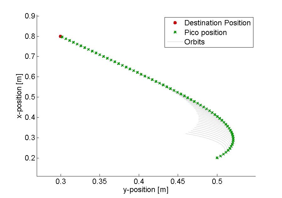
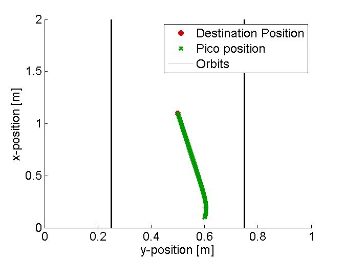
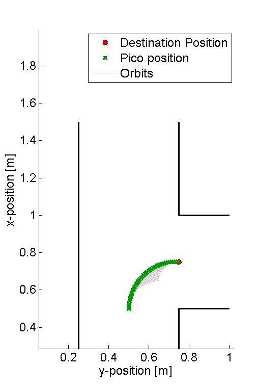
In the figure below, several examples of the working principle of the driving algorithm are shown. In the left figure, an extreem situation is sketched, such that one can clearly see the calculated orbits and the driving path. Such a situation is not likely to happen in the context of this project. The middle figure shows how the driving algorithm can be used to reallign the Pico when it is of center, and the right figure shows how corners can be taken by the Pico. In this latter situation, no intermediate destination points are needed, but are still an option.

Extreem example of the driving algorithm

Realigning example of the driving algorithm

Cornering example of the driving algorithm

Implementation in C++

As a result of the simplicity of the algorithm, the mere use algebraic functions and the few input information needed, the implementation in C++ can be rather easy. An overview of the code can for instance be given by:

Algorithm: Driving towards a destination point
    Input: Relative destination point (x,y) with respect to the Pico and its orientation
   Output: Translational and rotational constant velocities from driving the Pico

    Initialize: set the destination point to zero (relative to the Pico)

    while( ros::ok() ) {
       if destination message is received {
          Set relative destination point as the new destination
       } else {
          Calculate relative destination point by using the previous destination point
       }

       if [math]\displaystyle{ L_{d} }[/math] >= 0.01 {
          Calculate the orbit path and velocities
       } else {
          Set the velocities and the relative destination point to zero
          Realign the Pico with the lasers such that its driving direction is again parallel to the walls
       }

       Send velocities to the base
    }

Arrow Detection

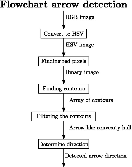
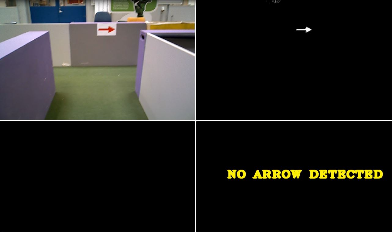
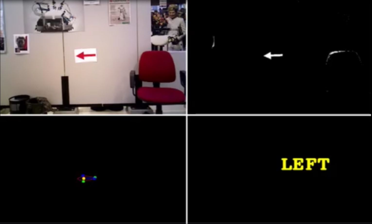
In order to drive to the corridor faster, it is useful to detect the various arrows in the corridors, guiding the pico towards the exit. Hereto, a separate node has been developed, which can work parallel to all the other nodes, to detect and interpret these arrows. In the figure to the below to the left, one can see a flowchart of the algorithm used for detecting the arrows. The various aspects for this detection are here below more elaborated.

Detecting the red objects

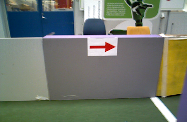
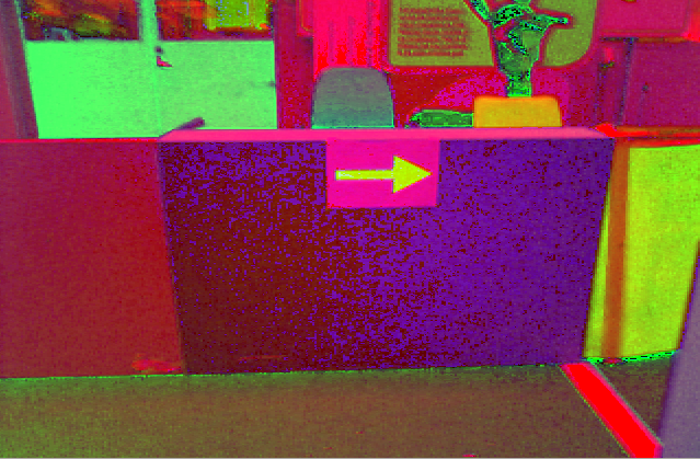
As it is given that the arrows to be detected are red, a first and obvious step is to detect the red objects in the image. From the pico camera one receives a color image in the RGB format, see for example the left figure below. However, it is easier to filter the image by a certain color when the image is in HSV format. The reason for this is that then the OpenCV function inRange can be used. As a result, the RGB image from the pico is first converted to this HSV format using the OpenCV function cvtColor, see the middle figure below for the result.

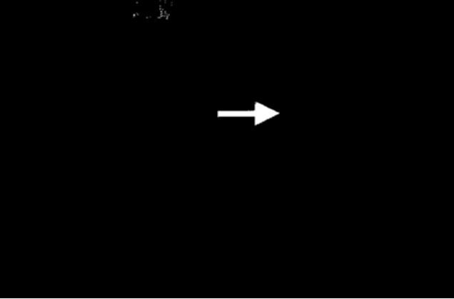
Subsequently, the HSV image is used to extract only the red objects in the image. In the HSV color spectrum handled by OpenCV, red is the color with the hue value equal to 0 or 180, hence slightly darker red lays in the range H = 170-180, while a lighter red color has an hue value H = 0-10. As a result, using only one threshold values to filter the image with may result in missing red objects. Therefore, to ensure all the red arrows are seen, the HSV image is filtered twice with the inRange function, and the results of both filters are added up. The resulting image is a socalled binary image, which only exists of white and black pixels, where the white pixels represent the red detected objects, see the most right figure below.

RGB image

HSV image

Binary image

Finding the arrow

Since multiple red objects could exist in the original RGB image, only filtering on the red color is not enough to detect the desired arrow. Therefore, the resulting binary image is filtered, to get rid of the unwanted red objects. Hereto, contours are used to determine the shape of the various detected red objects. In the binary image, contours are calculated around each object, which essentially matches the outer edge of the object. Now a first filter step can be applied, as the area of the contours can be calculated using the function contourArea. By demanding that the area must be larger than a certain threshold value, smaller detected objects can be eliminated from the binary image. However, choosing this area value too large will result in a late or even no detection of the arrow. As a result, only using the area filter will not be enough to eliminated all the unwanted red objects.

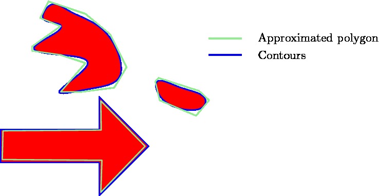
Therefore, all the found contours are approximated by a polygon using the approxPolyDP function in OpenCV. As the arrow has a standard shape, one knows that the approximated polygon will contain 7 vertices (or close to that number), while random red objects will have many more or less. This is illustrated in the figure to the right, where one can see a good approximated arrow, a contour which needs a high degree polygon for the approximation and a contour which only needs a low degree polygon for the approximation. By using this polygon approximation, one can actually get rid of must of the unwanted red objects, however, this filtering method is not waterproof, and hence more filtering steps are needed.

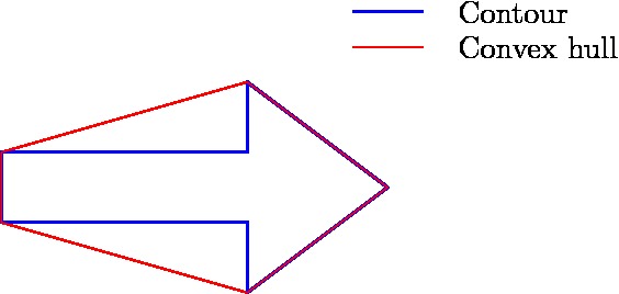
As a result, the principle of convex hulls is used as a next step to filter the binary image. For each of the remaining contours, a convex hull is calculated, which is the smallest convex set containing all the points of the detected object. In the figure below, the convex hull for the arrow is shown. As it can be seen, the contour and the convex hull have many similarities, however they differ in an essential point, the area they span. More precisely, when determining the ratio between the area of the contour and the area of the convex hull, for the arrows to detect it holds that [math]\displaystyle{ \frac{\text{area contour}}{\text{area convex hull}} \approx 0.6 }[/math], which is quite a specific number for the arrow. Therefore, as a final filtering step, this ratio is used to eliminate the final unwanted red objects. By combining the three main filtering steps, one can ensure that the only remaining contour in the binary image is the contour belonging to the arrow to be detected.

Determine the direction

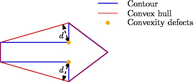
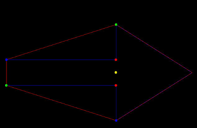
As the binary image has now be filtered such that only the contour of the arrow is remaining, one can start focusing on determining the direction the arrow is pointing. Hereto, again the principle of the convex hull is used, or more precisely, the principle of convexity defects. Convexity defects are in principle the points which have the largest deviations from the hull with respect to the contour. In the figure below on the left, one can see what the convexity defects are for the arrow, if the search depth [math]\displaystyle{ d }[/math] is choosing high enough. These convexity defects can then be used determine the midpoint of the arrow. The direction in which the arrow is pointing subsequently determined by measuring the amount of contour points to the left and right of this midpoint. As the arrow pointing part will contain many more points then the rectangular part of the arrow, the direction can thus be easily qualified. An overview of the contour, the convex hull, the convexity defects, and the midpoint as calculated by the algorithm can be seen in the figure below to the right.

Results

Below one can find several Youtube videos which demonstrate the working principle of the arrow detection algorithm.

SLAM

To be able to tackle any maze the use of Simultaneous localization and mapping is considered. When for example an arrow is detected and followed, it is possible to get stuck in a loop in the maze. Slam is a technique, that makes it possible to make an accurate estimate of the position of the robot relative to a certain point. This makes it also possible to make a map of the environment because all detected objects can be stored relatively to a certain point.

How slam works

For slam to work properly two sensors are used. First the odometry sensor, which estimates the position and orientation over time, relative to the starting location. This sensor however is sensitive to errors due to the integration of the data over time, this will therefore not be accurately enough to determine the position of the robot. So a second sensor, the laser-scanner, is used to help to improve this estimation. Slam works in different steps visualized in the figure below. The triangle represents the robot an the circles represent the landmarks.

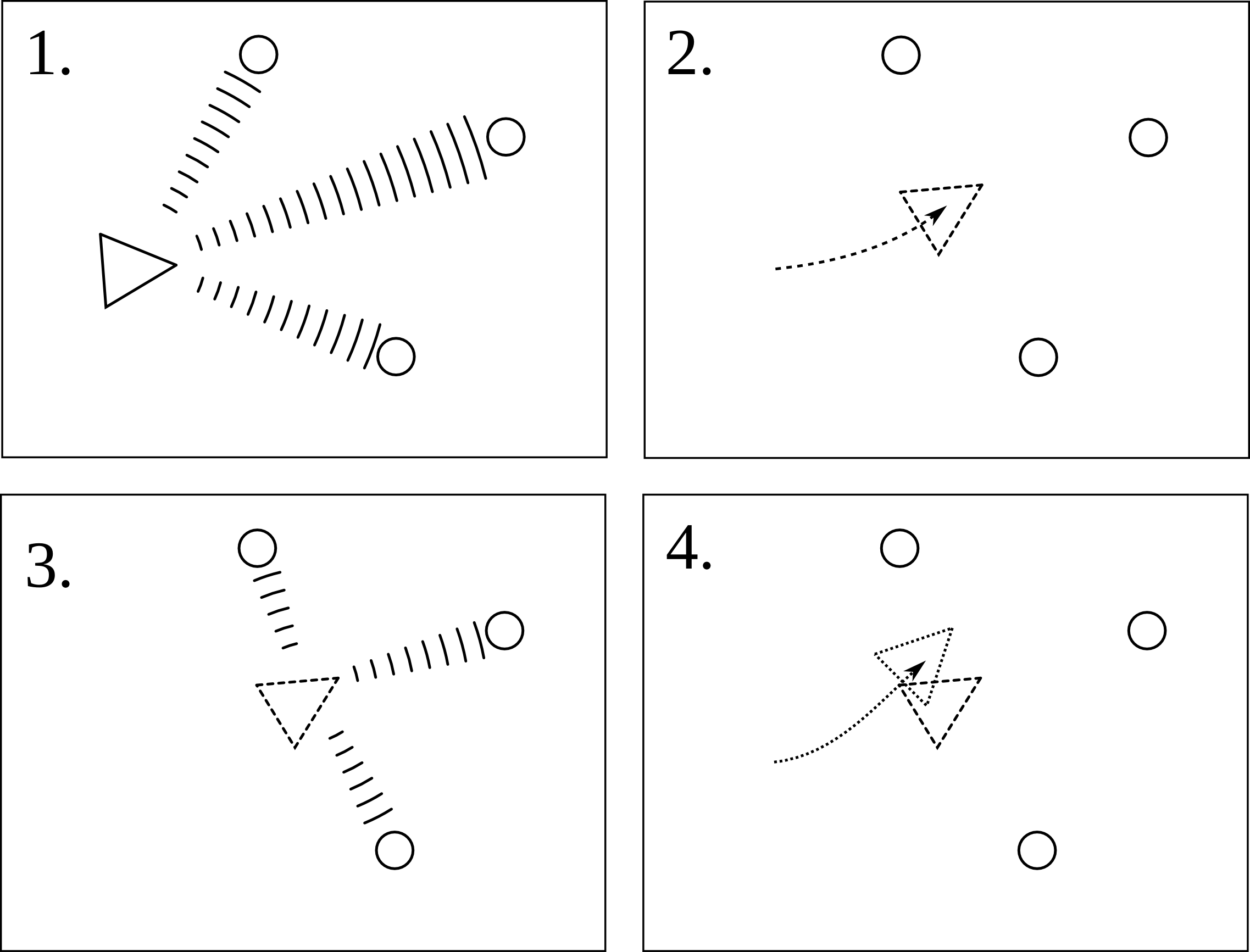
1. First the landmarks are detected using the laser-scanner. The landmarks could in this case be the walls and/or corners of the maze. The position of these landmarks are then stored relative to the position of the robot.

2. When the robot now moves the position and orientation is estimated by the odometry sensor, so the robot now 'thinks' that it is here.

3. The new locations of the landmarks relative to the robot are determined, but it finds them at a different location then where they should be, given the robots location.

4. The robot trusts its laser-scanner more then it trust its odometry, so now the information of the landmark position is used to determine where the robot actually is. Eventually also this new position is not the exact position of the robot because also the laser-scanner is not perfect, but the estimation is much better than relying on the odometry alone.

Gmapping

In ros there already is a package, called Gmapping, available which builds a map using SLAM. So this will be used to obtain the position of pico. Because a map is also provided, it might also be possible to use this map for finding walls and corners, and therefor detect the junctions. When using gmapping on pico the most important part is to determine the right parameters to get the most accurate results.

Algorithm

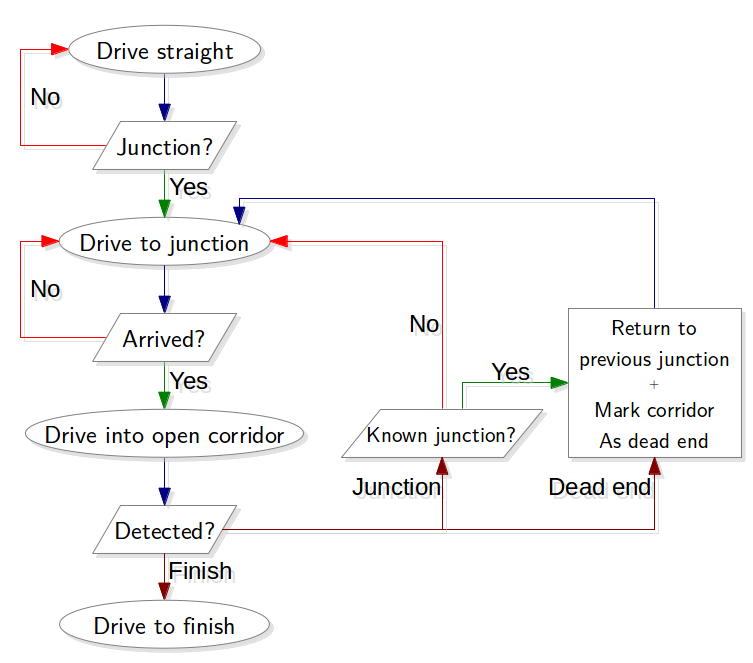
The advantage of SLAM is now that it is possible the store the position of objects relative to a certain point. This will be used to store the position of every junction that is encountered. Secondly for each junction every corridor is marked as: entered, open or dead-end. When then a junction is crossed again, this information is used to determine which exit will be taken and the information can then be updated. Below an algorithm, that can be used, is visualized. In this algorithm starts with finding a junction, when it finds one the robot will start to drive to that junction. Then it will choose when of the open corridors, for this an optimal order needs to be determined, for example always the most left corridor, or the information delivered by an arrow can be used. When the robot drives into a corridor it will now not only start to detect a junction, but also a dead-end and a finish. When the finish is found the robot can drive out of the maze. When a dead-end is detected the robot will return to the previous junction and mark the corridor as a dead-end. And when a junction is found the robot will drive to that junction and the algorithm starts again, unless the found junction is already encountered, which will then be treated as a dead-end. This algorithm should be able to find the exit without getting stuck in a loop.

Implementation of gmapping

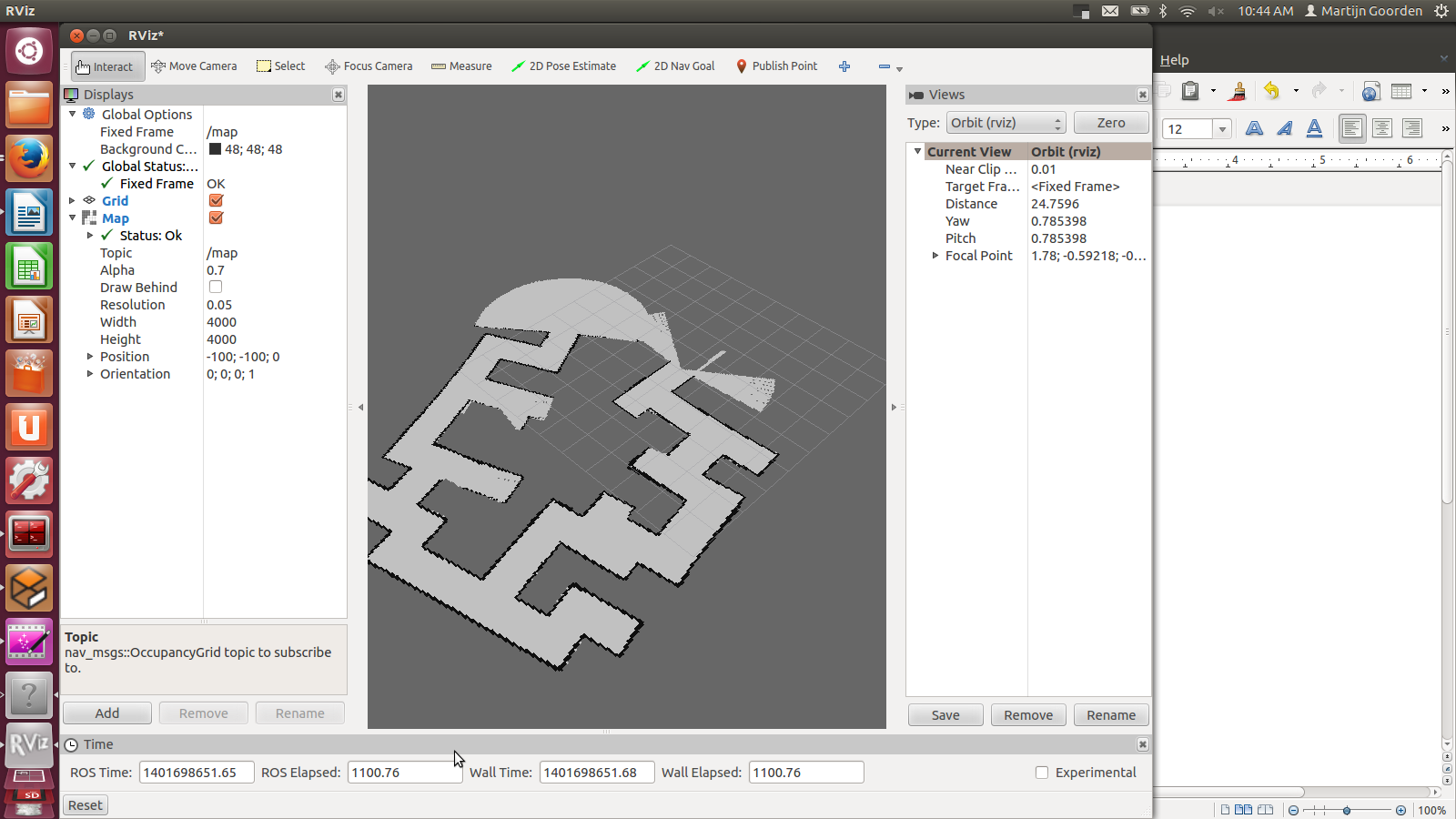
In the video below (click on the picture to be redirected to YouTube), a succesful implementation of gmapping is shown. The gemapping node is launched with the following parameters:

rosrun gmapping slam_gmapping scan:=/pico/laser _odom_frame:=/pico/odom _base_frame:=/pico/base_link _maxUrange:=2.0 _map_update_interval:=2.0 

First, the default frames of scan, odom_frame and base_frame need to be changed with the correct pico frames. Next, the maximum used range is set to 2.0 m. Finally, the update interval of the map is set to 2.0 s. A lower update interval requires more computation power. The video shows also that the generated map may contain errors. When, for example, the omniwheels slip, the odometry data is not perfect accurate any more. This results in a map with cornes less than or more than 90 degrees. gmapping corrects these errors if the robot drives a second time through a corridor. But in the perfect case, Pico finds the exist by driving only onces through every corridor.

Corridor competition

For the corridor competition, a step by step approach has been developed in order to steer the Pico robot into the (correct) corridor. Hereto, several subproblems have to be solved in a certain order as information of a subproblem is often needed to solve the next subproblem. The following subproblems can be distinguished:

1. Corridor detection. With the aid of the various sensors of the Pico, the corridor has to be recognized, i.e. the corners of the corridor must be known.
2. Path planning. By using the obtained information on the corridor, path planning can be used to guid the Pico into the corridor. Hereto, several way points are used.
3. Drive. Destination points have to be translated into a radial and tangential speed, which can actually drive the Pico.
4. Wall detection. For safety, an overruling program is needed which detects if the Pico is to close to any wall and if so can steer away from this wall.

26.8