Embedded Motion Control 2014 Group 1
Group Info
| Name: | Student id: | Email: |
| Groupmembers (email all) | ||
| Sander Hoen | 0609581 | s.j.l.hoen@student.tue.nl |
| Marc Meijs | 0761519 | m.j.meijs@student.tue.nl |
| Wouter van Buul | 0675642 | w.b.v.buul@student.tue.nl |
| Richard Treuren | 0714998 | h.a.treuren@student.tue.nl |
| Joep van Putten | 0588616 | b.j.c.v.putten@student.tue.nl |
| Tutor | ||
| Sjoerd van den Dries | n/a | s.v.d.dries@tue.nl |
Meetings
Weekly meetings are planned during the course. Every Wednesday a standard meeting is planned to discuss progress with the group and with the tutor. Presentations from these weekly meetings can be found with the presentation links below. Important meeting decissions can be found with use of the meeting liks below. Next to the standard weekly meetings evening meetings are planned to work as a group on the software design.
Time Table
Fill in the time you spend on this course on Dropbox "Time survey 4k450.xlsx"
Planning
Week 1 (2014-04-25 - 2014-05-02)
- Installing Ubuntu 12.04
- Installing ROS
- Following tutorials on C++ and ROS.
- Setup SVN
- Plan a strategy for the corridor challenge
Week 2 (2014-05-03 - 2014-05-09)
- Finishing tutorials
- Interpret laser sensor
- Positioning of PICO
Week 3 (2014-05-10 - 2014-05-16)
- File:Presentatie week 3.pdf
- Starting on software components
- Writing dedicated corridor challenge software
Week 4 (2014-05-17 - 2014-05-25)
- File:Presentatie week 4.pdf
- Finalize software structure maze competition
- Start writing software for maze competition
Week 5 (2014-05-26 - 2014-06-01
- Test first maze competition software in practice
- Determine bottlenecks for maze competition
- Start with arrow detection
Software architecture
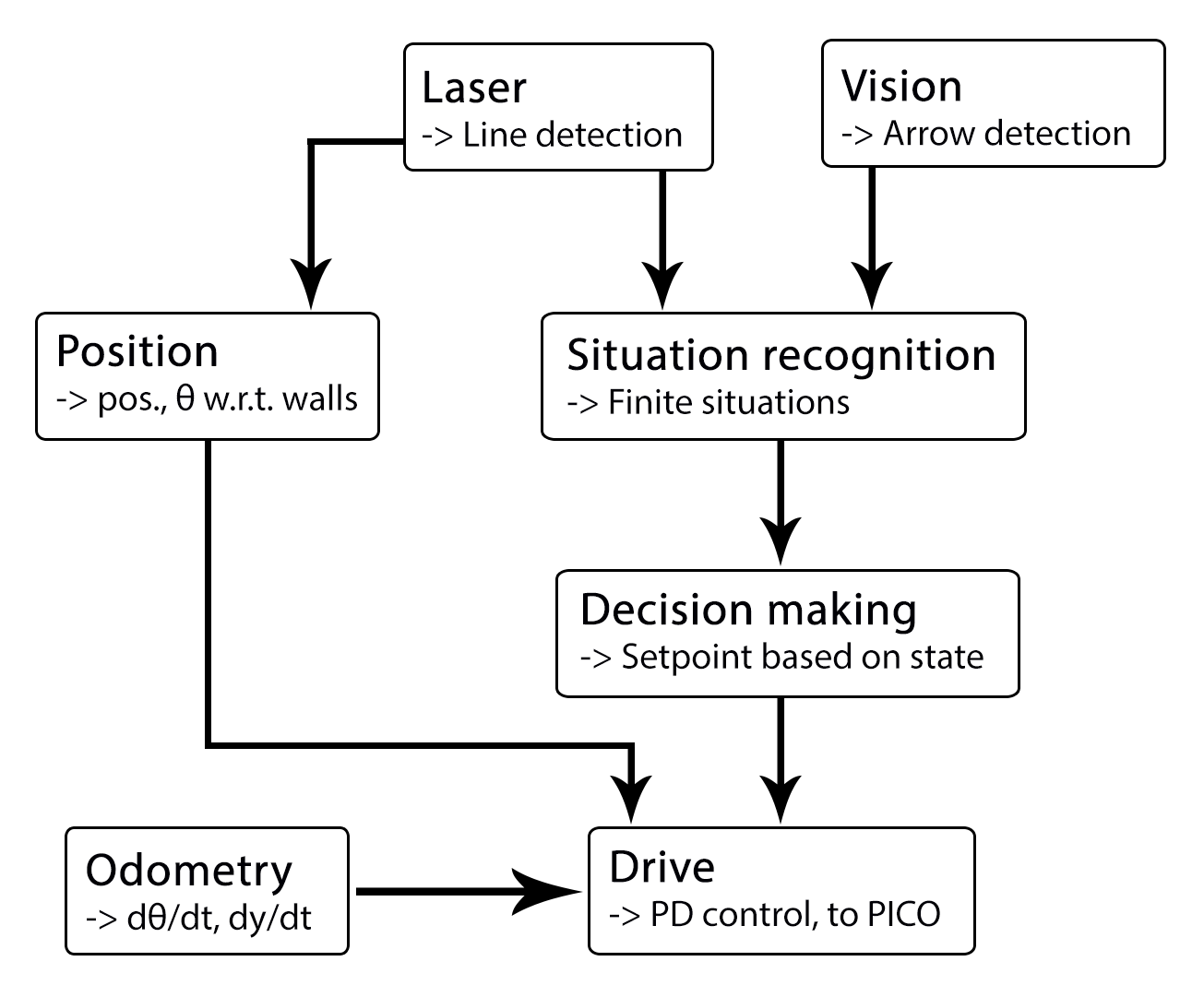
We decided to use a architecture as seen as the following figure:

The components with their respective functions and in and outputs are listed here + who wil work on it:
| node | subscibes topic: | input | publishes on topic: | output | Description |
| Line detection - Sander | - | laser scan | /pico/line_detection | lines consisting out of start and end point (x_1,y_1),(x_2,y_2) etc. | transformation of raw data to lines by use of hough-transform |
| Position - Richard | line coordinates | (X_left, X_right, Y, theta) also named 'relative position' | Determine distance to wall to left, right and front wall. Also determines angle theta with respect to the corridor. | ||
| Arrow detection | camera | Arrow left of right | determine if pico sees an arrow and in what direction. | ||
| state recognition - Joep | lines, vision, relative position | an integer of whitch state is recognized | recognize situation and transform this to one of the states. | ||
| setpoint generator - Wouter | state, relative position | speed and position | Create setpoint for position of pico by use of state. (determine wanted position and speed). | ||
| Drive - Marc | setpoint, relative position | x,y,thata (Moving pico) | make sure that pico is positioned centered if this is needed and turn when needed.
|
Line detection - Sander
inputs: --
function: transformation of raw data to lines by use of hough-transform
output: lines consisting out of start and end point (x_1,y_1),(x_2,y_2) etc.
convert laser data to points (x,y)
use hough transform
filter lines
data output format: (richard + sander)
topic: /pico/lines
msg: lines
relative distance - Richard
input topic: /pico/lines
function: Determine distance to wall to left, right and front wall. Also determines angle theta with respect to the corridor.
output: (Y_left, Y_right, X, theta)
output topic: /pico/dist
msg: dist
The angle theta can be calculated with the next fomula:
[math]\displaystyle{ \theta = atan((y2-y1)/(x2-x1)) }[/math]
the position perpendicular to the line/wall is calculated with the next formula:
[math]\displaystyle{ X_r = x2 - ((y2-y1)/(x2/x1))*y2*sin(\theta_1) }[/math]
[math]\displaystyle{ X_l = x4 - ((y4-y3)/(x4/x3))*y4*sin(\theta_2) }[/math]
theta is average of left and right or only left or right depending on situation
Drive - Marc
inputs: setpoint, relative position
function: make sure that pico is positioned centered if this is needed and turn when needed.
outputs: (Moving pico)
Situation - Wouter
inputs: lines, vision
Lines can be categorized in two types of lines:
Longitudinal lines: y-coordinates of begin and end point are similar
Lateral lines: x-coordinates of begin and end point are similar
Situations to be recognized:
- inbetween two walls
No obstacles in front, no lateral line detected within X meter.
2 longitudinal lines are detected.
- Junction
3 lines are detected. From which two are longitudinal lines and one is lateral within (X meter).
Detect direction of juction by comparing the x -values of the longitudinal lines with the x-value of the lateral line.
Left junction: When the x value of the left line (the line with the smallest Y values) is 'minimum corridor width' smaller then the x value of the lateral line a gap on the left side is recognized.
Right junction: When the x value of the right line (the line with the smallest Y values) is 'minimum corridor width' smaller then the x value of the lateral line a gap on the left side is recognized.
- Dead end
3 lines are detected. From which two are longitudinal lines and one is lateral within (X meter).
Detect direction of dead end by comparing the x -values of the longitudinal lines with the x-value of the lateral line. When the x values of both longitudinal lines are similar to those of the lateral line a dead end can be recognized.
- T junction: 3 situations named T-right, T-left, T-right-left.
T-right: 3 longitudinal lines are detected, 1 lateral lines detected on the right side of pico.
T-left: 3 longitudinal lines are detected, 1 lateral lines detected on left side of pico.
T-right-left: 2 longitudinal lines are detected: 4 lateral lines are detected
- X junction
4 longitudinal and 4 lateral lines are detected
State generator - Joep
input: Situation, relative position
input topic: /pico/sit
function: Create setpoint for position of pico by use of state. (determine wanted position and speed).
output:
output topic: /pico/
msg:
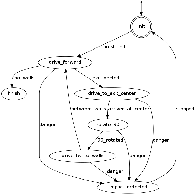
PICO states corridor challenge
For the robot, the internal states can be visualized as in the following figure:
