Embedded Motion Control 2014 Group 11

Go back to the main page.

Group Members

Name:	Student id:	Email:
Groupmembers (email all)
Martijn Goorden	0739273	m.a.goorden@student.tue.nl
Tim Hazelaar	0747409	t.a.hazelaar@student.tue.nl
Stefan Heijmans	0738205	s.h.j.heijmans@student.tue.nl
Laurens Martens	0749215	l.p.martens@student.tue.nl
Robin de Rozario	0746242	r.d.rozario@student.tue.nl
Yuri Steinbuch	0752627	y.f.steinbuch@student.tue.nl
Tutor
Ramon Wijnands	n/a	r.w.j.wijnands@tue.nl

Time survey

The time survey of this group will be hosted on a Google drive. Therefore, all group members can easily add information and anyone can see the up-to-date information. The document can be accesed by clicking this link: time survey group 11

Planning

Week 1 (28/4 - 4/5)

Finish the tutorials, including

• installing Ubuntu,
• installing ROS
• installing SVN
• get known with C++
• get known with ROS

Week 2 (5/5 - 11/5)

Finish the tutorials (before 8/5)

• Setting up an IDE
• Setting up the PICO simulator

Work out subproblems for the corridor competition (before 12/5)

Comment on Gazebo Tutorial

When initializing Gazebo, one should run the gzserver comment, however, this can result in a malfunctioning program, i.e. you will get the following message: Segmentation fault (core dumped). The solution for this is to run Gazebo in debugging mode (gdb):

1. Open a terminal (ctrl-alt-t)
2. Run:

   gdb /usr/bin/gzserver

   when (gbd) is shown, type run and <enter>
3. Open another terminal (ctrl-alt-t)
4. Run:

   gdb /usr/bin/gzclient

   when (gbd) is shown, type run and <enter>

Comment on running Rviz

Simular to the Gazebo tutorial, the command rosrun pico_visualization rviz can also result in an error: Segmentation fault (core dumped). Hereto, the solution is to run Rviz in debugging mode:

1. Open a terminal (ctrl-alt-t)
2. Run:

   gdb /opt/ros/groovy/lib/rviz/rviz

   when (gbd) is shown, type run and <enter>

Moreover, in order for the camera to work properly, in the Displays view on the left change the Fixed Frame.

Corridor competition

For the corridor competition, a step by step approach has been developed in order to steer the Pico robot into the (correct) corridor. Hereto, several subproblems have to be solved in a certain order as information of a subproblem is often needed to solve the next subproblem. The following subproblems can be distinguished:

1. Corridor detection. With the aid of the various sensors of the Pico, the corridor has to be recognized, i.e. the corners of the corridor must be known.
2. Path planning. By using the obtained information on the corridor, path planning can be used to guid the Pico into the corridor. Hereto, several way points are used.
3. Drive. Destination points have to be translated into a radial and tangential speed, which can actually drive the Pico.
4. Wall detection. For safety, an overruling program is needed which detects if the Pico is to close to any wall and if so can steer away from this wall.

Corridor detection

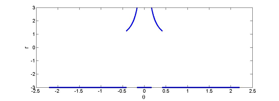
First a horizon R is being set. Every value r(i) > R is being replaced by r(i) = -R. This can be seen in the figure below where R=3.

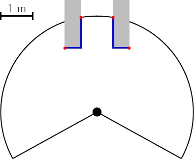
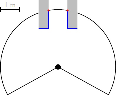
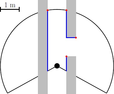
Then the change in the radii are evaluated: dr = r(i+1) - r(i). When dr>R then r(i+1) is saved, when dr<-R then r(i) is saved. A set-point can be set in between the two corridor points. However there are 4 points in this situation (see figure left below), the two central represent the corridor. Any outer point can be removed from the set (figure center below), this results in at least one pair of 2 corridor points (figure right below shows the possibility of multiple corridor point pairs)

Driving the Pico

The Pico needs to drive towards the first destination point of the resulting path planning. There are various ways to achieve this by using its two independ velocity componements, namely the translational speed [math]\displaystyle{ \dot{x} }[/math] and its rotational speed [math]\displaystyle{ \dot{\theta} }[/math]. One could for instance first rotate the Pico in the right direction, to subsequently just drive forwards until the destination is reached. However, this can be a time consuming task as the Pico has to stop each time a correction on the direction has to be made. Moreover, when a corner needs to be taken, mutlitple waypoints are necessary to guid the Pico. Therefore, an alternative algorithm is developed, which can react more quickly on directional changes and steers the Pico as fast as possible towards its destination. To concept of this algorithm is shown in the figure to the left.

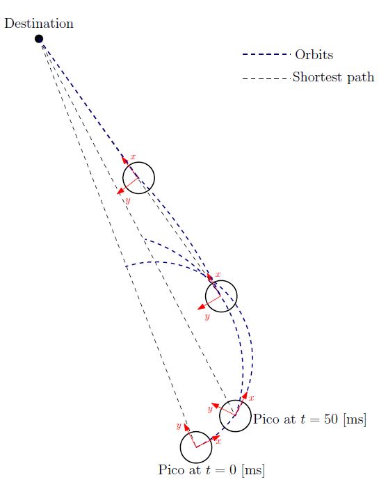
Here an extreem situation is sketched, to fully illustrated the functioning of the method. In the figure, the pico is shown at various moments in time, where the driving direction (or facing direction of the Pico) is the relative x-direction. Moreover, a destination point is shown in absolute coordinates, however, one must keep in mind that the information fed to the algorithm is the relative destination with respect to the Pico and all calculations are performed on this relative coordinate set.

The general idea of the algorithm is as follow: The shortest distance from the Pico to its destination would simply be a linear path. However, as the pico often does not face that direction, it is not possible to drive with the given velocity componements along this linear path. On the contrary it is possible to descirbe orbit paths which get the Pico as fast as possible on that linear path (see the figure on the left). These orbits are described by:

[math]\displaystyle{ x(t) = \dot{r}t\cos{(\dot{\theta}t)} }[/math] and [math]\displaystyle{ y(t) = \dot{r}t\sin{(\dot{\theta}t)} }[/math]

One can do so by demanding that after a certain time [math]\displaystyle{ T }[/math], which is a function of the sampling time [math]\displaystyle{ T_{sample} }[/math] and the distance to the destination [math]\displaystyle{ L_{d} }[/math], i.e. [math]\displaystyle{ T = f( T_{sample}, L_{d} ) }[/math], the Pico has reached this linear shortest path. However, as the Pico moves, the shortest path to the destination changes. As a result, after each [math]\displaystyle{ T_{sample} }[/math] seconds, the orbits are recalculated as shown in the figure to the left, resulting in a smooth path towards the destination.

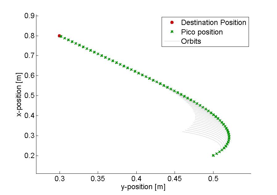
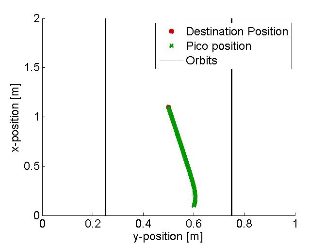
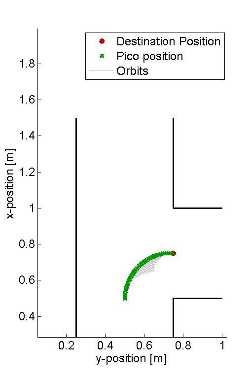
In the figure below, several examples of the working principle of the driving algorithm are shown. In the left figure, an extreem situation is sketched, such that one can clearly see the calculated orbits and the driving path. Such a situation is not likely to happen in the context of this project. The middle figure shows how the driving algorithm can be used to reallign the Pico when it is of center, and the right figure shows how corners can be taken by the Pico. In this latter situation, no intermediate destination points are needed.

Implementation in C++