Embedded Motion Control 2017 Group 6
About the group
| Name | Student ID | |
|---|---|---|
| Ties Hoenselaar | 0857112 | t.a.h.hoenselaar@student.tue.nl |
| Hasan Ilisu | 0852221 | h.h.ilisu@student.tue.nl |
| Laura de Jong | 0743679 | l.s.d.jong@student.tue.nl |
| Lars Moormann | 0861223 | l.moormann@student.tue.nl |
| Bas Straatman | 0777325 | s.r.t.straatman@student.tue.nl |
| Jeroen van der Velden | 0744957 | j.r.v.d.velden@student.tue.nl |
| Wouter Houtman | Tutor | w.houtman@tue.nl |
Introduction
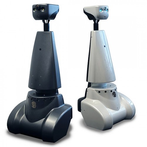
The most memorable part of the course Embedded Motion Control is the 'A-MAZE-ING PICO' challenge, in which software is designed for and implemented into autonomous robots. These autonomous robots, called Pico and Taco, should then be to able to solve a maze with the software in a real-life environment. A maze can contain loops, dead ends, open spaces and doors that automatically open and close.
Pico will be provided with a basic software layer to carry out primary functions, such as communication and movement. However, to succesfully complete the 'A-MAZE-ING PICO' challenge it is required to design robust software for the changing environment. Several software subsystems will be put to the test in an intermediate challenge. During this challenge, called the corridor competition, Pico must move through a corridor and take the first exit. With the results of the corridor competition and all its software subsystems Pico should be able to finish the maze challenge. The course Embedded Motion Control is concluded with an overall conclusion.
Software design
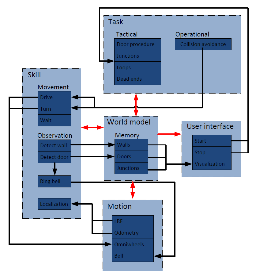
The ever-changing environment in reality requires the design of a robust software architecture. It is prefered to design this software architecture before actually programming, because it gives a clear understanding/agreement of the different functions from the start. The first step in creating the software architecture is to mention the requirements that have to be met in order to complete the corridor competition and the maze challenge. Pico should be able to finish these challenges succesfully by using most of its components. Secondly, a list of specifications will be given to accuratly describe the robot, corridor and maze. With these requirements, components and specifications it is then possible to define functions for the software architecture. The software architecture is completed by specifying the interfaces between task, skill, motion, world model and user interface. It is noteworthy to mention that the final software design in this section, which was also presented during our final presentation, is based on our initial design plan report and first presentation.
Requirements
To complete the corridor competition and maze challenge Pico has to meet the following requirements:
- Operate fully autonomous
- Avoid collisions with walls
- Robust against sensor disturbances and layout imperfections
- Update, compile, start and end software with single commands
- Corridor competition
- Move through a corridor that complies with the specifications
- Exit the corridor within the set time limit
- Recognize junctions
- Maze challenge
- Move through a maze that complies with the specifications
- Escape the maze within the set time limit
- Recognize junctions, loops, dead ends and doors
- Ring the bell at dead ends and doors
- Stand idle for a certain period of time
Components
The following components of Pico will be used to fulfill the requirements:
- Sensors
- Laser range finder (LRF) determines the distance to an object with a laser beam
- Wheel encoders (odometry) determine the position of Pico relative to a starting position
- Actuators
- Holonomic base with three omni-wheels to drive and turn
- Bell to request a door to open
- Computer
- Intel I7 processor
- Ubuntu 14.04 as operating system
Specifications
Pico, the corridor competition and the maze challenge are characterized by the following specifications:
- Pico
- Dimensions of 42 cm x 40 cm x 108 cm (LxWxH)
- Maximum translational speed of 0.5 m/s
- Maximum rotational speed of 1.2 rad/s
- Maximum amount of bell actions equal to the amount of doors plus dead ends
- Maximum idle time of 30 seconds
- LRF
- Located at ??
- Range of 0.1 to 30 m
- Accuracy of ± 10 mm
- Horizontal field of view of 270°
- Resolution of 0.25°
- Frequency of 40 Hz
- Odometry
- Located at ??
- Resolution of ??
- Frequency of ??
- Accuracy of ?? (negligible compared to the slip of the omni-wheels)
- Corridor competition
- Maximum of two attempts within 5 minutes total
- Penalty of 5 seconds or 1 attempt when slightly touching or bumping a wall
- Corners are approximately 90°
- Walls are approximately parallel to each other
- Distance between walls can range from 0.5 to 1.5 meter
- Distance from start to finish is between 1 and 10 meters
- Start is located between the walls in the main corridor
- Finish is located 0.3 meter inside a side corridor on either the left or right
- Main corridor has open ends
- Maze challenge
- Maximum of two attempts within 7 minutes total
- Penalty of 5 seconds or 1 attempt when slightly touching or bumping a wall
- Corners are approximately 90°
- Walls are approximately parallel to each other
- Distance between walls can range from 0.5 to 1.5 meter
- Distance from start to finish is unknown
- Start is located inside the maze, but outside a door area
- Finish is located on the boundary of the maze behind a door
- Can contain loops, open spaces and more than one dead end
- Contains one door and it is located at a dead end
- A dead end is between 0.5 and 1.5 meter wide and at least 0.3 meter long
- A door area is located in front of a door and is 1.3 meter long
- Door opens when Pico is inside the door area, stands still and sends a request
- Door starts opening within 2 seconds and is fully opened within 5 seconds
- Door opens to the left or right with approximately constant velocity
Functions
The requirements can be met with the given components and specifications by defining various functions for the software architecture. These functions typically use sensor information to determine the next actuator action, or compute a variable that is used by another function. When defining functions it is important that each function has a single and clear purpose. All the functions that are required to complete the maze challenge are visualized in a function flow chart. The colors in the function flow chart indicate how much functionality of a function is necessary to finish the corridor competition instead. This design saves time because every function used in the corridor competition is reusable for the maze challenge. The function flow chart starts every iteration with getting sensor data, and based on the state of the state machines a different part of the code is executed. A dashed line is used to illustrate which function can alter the state in a state machine. Furthermore, the main and sub state machines are initialized at the corridor, initiate and request state.
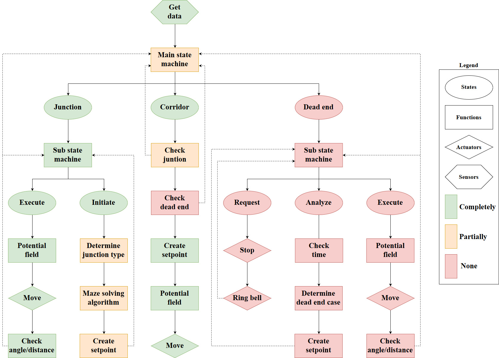
The role of each function will be clarified with three small scenarios. In the first scenario Pico is located at one end of a corridor and needs to move to the other end. Pico will do so by first getting sensor data from the LRF and odometry, and then entering the corridor state via the main state machine. The LRF data is then used to check whether there is a junction or dead end near Pico. This is not the case, so a setpoint is created in front of Pico. The setpoint and the location of the walls are then used to create a potential field. With this potential field Pico is able to move a small distance through the corridor while avoiding the walls.
In the second scenario Pico is located near a junction, but the junction has not yet been detected. Similar to the first scenario Pico will obtain sensor information, enter the corridor state and use the LRF data to determine if there is a junction or dead end near Pico. However, this time a junction is detected and the state of the main state machine is switched to the junction state. This switch ensures that Pico carries out the functions in the initiate sub state at the next iteration. Within the initiate sub state the type of junction is determined, a decision is made by the maze solving algorithm and a setpoint is created in the direction Pico needs to move. After the initiate sub state is carried out once, the state of the sub state machine is set to the execute sub state. The functions in the execute sub state are carried out every iteration until Pico has driven/turned sufficiently according to the odometry data. In other words, the main state machine and sub state machine are reset to their initial states when Pico is close to its setpoint.
In the third scenario Pico is located in a corridor with a dead end, and the the dead end has just been detected. This implies that Pico will carry out the functions in the request sub state at the next iteration. The request sub state ensures that Pico stops moving and that it rings the bell. After the request sub state is carried out once, the state of the sub state machine is set to the analyze sub state. The first function in the analyze sub state is used to wait a predefined amount of time for a possible door to open. When the time has passed the LRF data is used to determine whether it was a door or dead end. Based on its findings a setpoint is created in front or behind Pico in case of a door or dead end, respectively. After the setpoint has been created, the state of the sub stame machine is set to the execute sub state. Finally, the functions in the execute sub state are carried out every iteration until Pico has driven/turned sufficiently according to the odometry data.
Interfaces
Software subsystems
Junctions
Dead ends
Setpoints
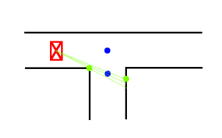
The setpoint detection function is used after the junction type is recognized and Pico has made a decision on which way to go. The function first finds the required corner points corresponding to the junction type and then converts the data into the correct setpoint data. The first figure on the right shows an example of a junction type and the required points to determine.
The green points in the figure represent the points pico will recognize. The blue points are the setpoints Pico will use to take the corner. The locations of the these blue points are calculated from the data of the green points.
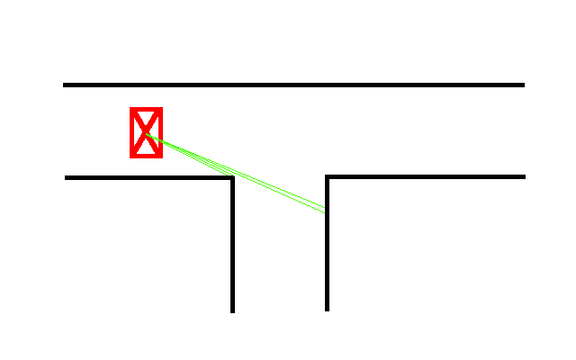
The left green point is the first point Pico will look for. To find this, it will go through a part of its laser data and compare the distances of subsequent data entries. In this for-loop, the distance of the current laser data (called i) and the distances of the three following data points (i+1, i+2, i+3) are compared. When the difference is higher than a set minimum (5 cm), Pico will recognize this as a gap in the sidewall and save the corresponding angle and distance. The left green point corresponds to the data point i, and the right green point is data point i+3. The second figure visualized this process.
Once the data of the green points is found, this data is converted into an offset in x and y direction. This offset is measured with Pico as origin, where the x-direction is the direction Pico is driving in, and the y-direction is perpendicular to this. The offsets are calculated by first determining the angle at which the data point lies, after which trigonometry is used to find the offsets. The equations below show the formulas used in the code.
- [math]\displaystyle{ \theta }[/math] = (laser.angle_min + laser.angle_increment * i_corner1) * 67.5 * [math]\displaystyle{ \pi }[/math] / 180
angle_min is the smallest angle Pico can see, angle_increment is the difference in angle between two data points, i_corner1 is the data entry corresponding to the left green point.
- [math]\displaystyle{ }[/math] setpoint.x = (dist1+dist2) / 2 * cos([math]\displaystyle{ \theta }[/math])
dist1 and dist2 are the distances in the laser data of the left and right green points respectively.
- [math]\displaystyle{ }[/math] setpoint.y = (dist1+dist2) / 2 * sin([math]\displaystyle{ \theta }[/math])
The lower blue point in the first figure is then determined by calculating the point exactly between the two green points. The data for this blue point is once again saved as an offset in x- and y-direction. The offsets of the upper blue point is then simply calculated by taking the same x-offset as the lower blue point, and setting the y-offset to 0.
This example is obviously only applicable when Pico needs to take a turn to the right. The same procedure can however be used when the turn is to the left, but the data range used to find the setpoints is then adjusted.
The final option for Pico is to go straight at a junction. The third figure shows where the setpoints are placed in that scenario. The calculation of the setpoints is done in the same way as before.

Potential field
Pledge algorithm
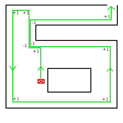
To find the exit of the maze the Pledge algorithm is chosen. The Pledge algorithm is suitable for maze problems where the starting point is within the maze and the exit is at the border of the maze. The modified wall following algorithm has a preferred direction which allows the robot to circumvent obstacles and directs the robot towards the outer walls of the maze. By tracking the number of perpendicular turns the algorithm keeps track of the direction. The Pledge algorithm is chosen because it is suited for the problem and simple to implement in the code. The algorithm can be based on either a left- or right-hand wall follower. There is no significant difference between the two versions. Which version can find the exit faster depends on the maze and the location of the entrance and exit. Since the maze is unknown, the choice to use a right-hand wall follower in the maze challenge is arbitrarily.
The rules for the right-hand Pledge algorithm are:
- When the counter is in the preferred direction; when the counter is 0: try to go straight (+0), then try to go left (+1), or else, turn around (+2).
- When the counter is not in the preferred direction; when the counter is not 0: try to go right (-1), then try to go straight (+0), then try to go left (+1), or else, turn around (+2).
An example of the algorithm can be seen on the right. The algorithm is implemented in the 'make decision' function by applying the rules to the different junction types. For every junction type and counter setting(zero or non-zero), the decision which direction to go is predefined. In another function the counter is updated, depending on de selected direction.
Visualization
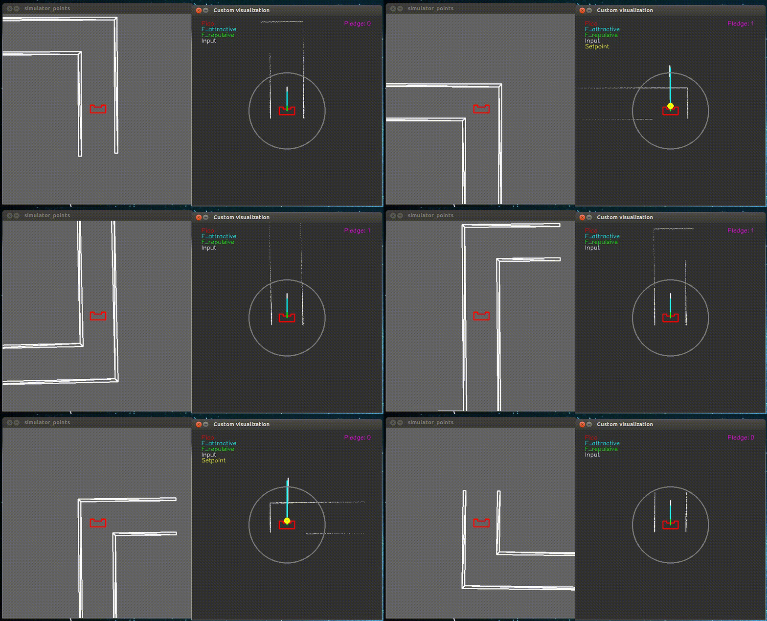
A custom visualization has been made to show the forces of the potential field, the maximum viewing range of PICO and the location of the setpoint. The function “show_canvas” must be called to update the visualization. This function has multiple inputs which are: the laser-data of PICO, the forces class and the location of the setpoint.
In the video below on the right the custom visualization is shown with in the top left corner a small legend and on the top right the pledge counter. The white dots represent the laser data and the gray circle around PICO is the maximum viewing range.
The three forces which are shown are: the attractive force (in blue), the repulsive force (in green) and the total force, which is the sum of the attractive forces and the repulsive forces (in white). These forces are returned by the potential field in a class called “forces”. The reason for this is that a function can only return one value or class in our case.
A code snippet of the code used for the visualization can be found here.
 |
Corridor competition
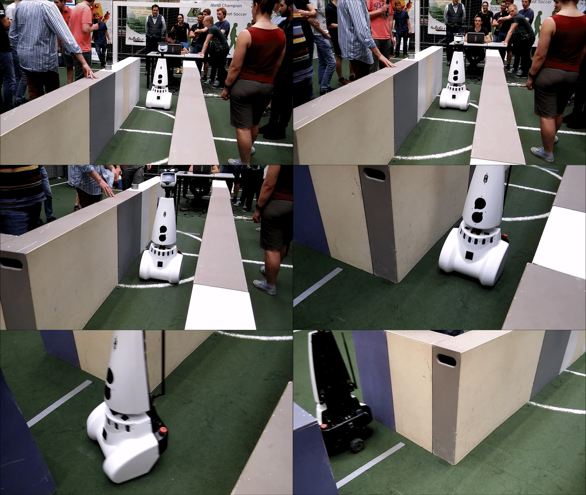
The purpose of the corridor competition is to test part of the software architecture halfway through the course. During this intermediate challenge on the 24th of May Pico had to move through a corridor and take the first exit. The location of the exit and dimensions of the corridor were not given in advance, but were determined by the organisation at the time. For the first attempt we used a version of the software that was actually tested on Pico the day before. During this test it became clear that this version had sometimes difficulties making a turn at the T-junction. Nonetheless, we decided to use this version of the software and hoped for the best. The performance of Pico during its first attempt in the corridor competition is shown in the following video.

In this video it is visible that Pico is able to correctly move through the corridor, but that it pauses before taking the wrong exit. Pico was standing still at the T-junction because it was unable to create a setpoint in the initiate sub state. This issue arises from
