Embedded Motion Control 2015 Group 2
Go back to the main page.
|
|
 |
Group Members
| Name: | Student id: | Email: |
| Groupmembers (email all) | ||
| Wouter Kuijpers | 0864565 | w.j.p.kuijpers@student.tue.nl |
| Carel Wechgelaer | 0874762 | c.a.wechgelaer@student.tue.nl |
| Natalia Irigoyen | 0929175 | n.irigoyen.perdiguero@student.tue.nl |
| Stephanie Dávalos | 0925756 | s.davalos.segura@student.tue.nl |
| Georgi Hristov | 0931293 | g.s.hristov@student.tue.nl |
| Paul Padilla | 0926256 | g.p.padilla.cazar@student.tue.nl |
| Garbí Singla | 0932046 | G.Singla.Lezcano@tue.nl |
| Tutor | ||
| Luis Ferreira | n/a | L.F.Bento.Ferreira@tue.nl |
Initial Design
More information about the Initial Design can be found on the Intial Design-page. Here you can also find the Design Document and the Initial Presentation which was presented at 6th of May.
Corridor Competition
On the 13th of May 2015 the Corridor Competition was scheduled. Videos of our both attempts to reach the finish of the corridor can be viewed by clicking on the two pictures below
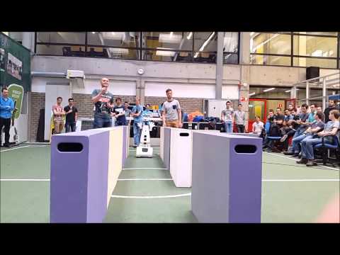 |
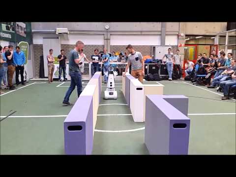 |
Analysis First Try
- Keeping Minimum Distance-algorithm: performs oké, an initial limit estimation was used ensuring that the robot keeps a safe distance to the wall.
- Turning: after making a 90 degree turn the coordinator presumably switched back to normal mode, then it saw a new end of the corridor on the left and wanted to turn immediately. In this case the coordinator had to be overwritten by first driving forward without the possibility of again turning.
Analysis Second Try
- Keeping Minimum Distance-algorithm: performs oké, an initial limit estimation was used ensuring that the robot keeps a safe distance to the wall.
- Turning: we do not know what went wrong here. So far we have also not succeeded recreating the same behavior in the simulator.
Lessons Learned
- A new algorithm is needed for keeping the minimum distance to the wall, this algorithm causes a large variation in the robot's orientation. In designing this new algorithm use can be made of the algorithm as a basis.
- A new algorithm is needed to detect possible turns or, in the real maze, intersections and T-junctions. In designing this new algorithm use can be made of the algorithm as a basis.
Composition Pattern
On the 27th of May the Composition Pattern presentation was given in the EMC lecture. In this presentation the (slightly revised) Task-Skill-Motion-framework was presented and the mapping from this to the Composition Pattern Hierarchy.
The slides of the presentation can be found here:
- Composition Pattern Presentation - File:Presentation 27052015.pdf
Final Design
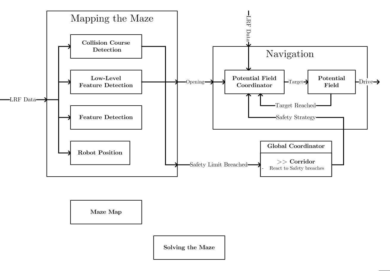
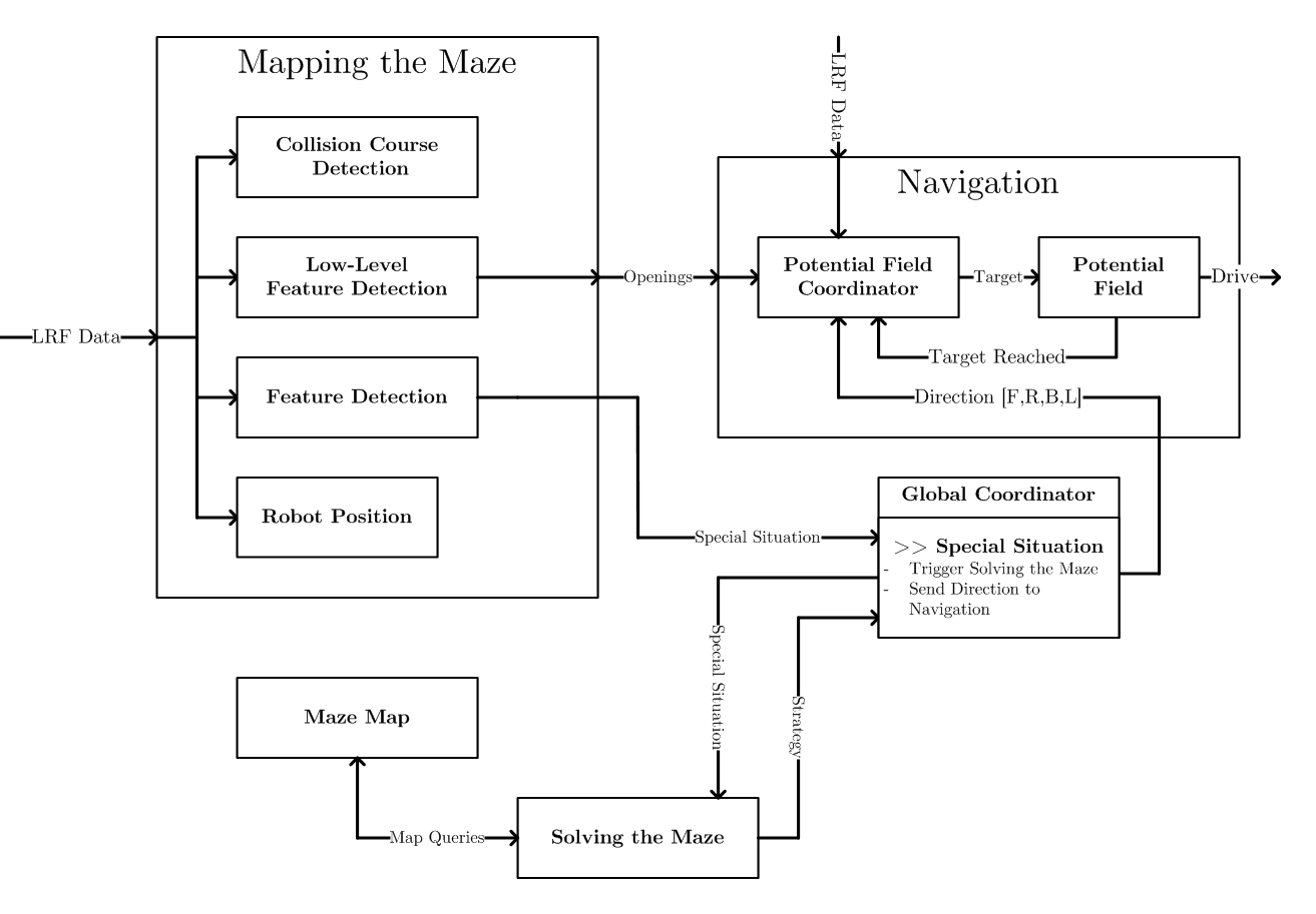
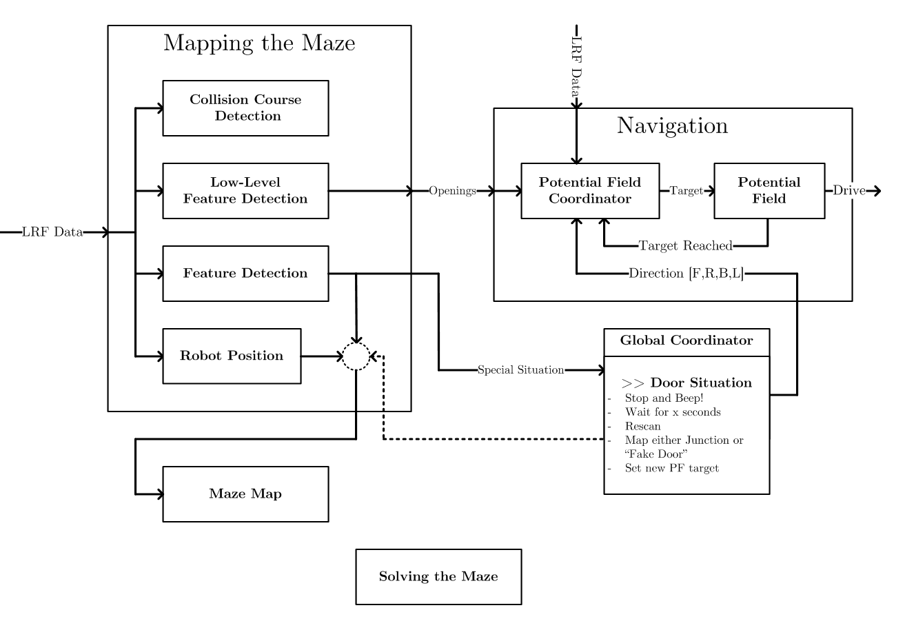
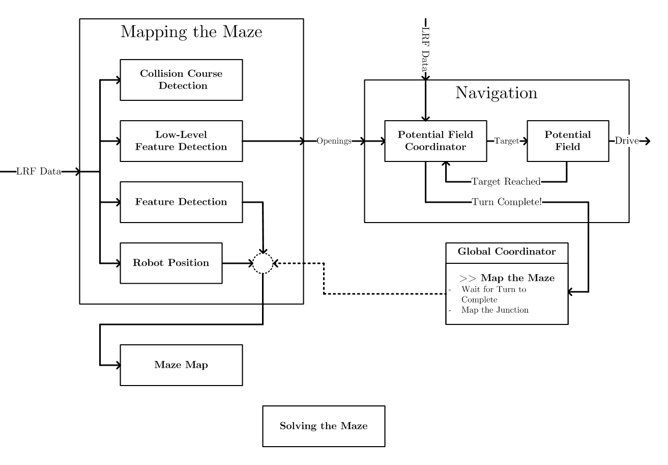
For the Final Design of the PICO software, the software structure was broken down into four situations: straightforward navigation, detection of a special situation, mapping the junction and detecting a door. In each of these four situations the overall software flow is described using the four software schematics shown on the left and the right of this of text.
The overall flow in the diagram is mostly controlled by the general coordinator which will be explained in more detail near the end of this page. The functionality contained in each of the separate functional components will be described first. Each of the functional components will briefly summarize the method used and then expand on the implementation of it. At the end, each functional component will demonstrate the working of the actual software algorithm.
Most of the functional components also present (part of) the code in pseudo-code in their description but also parts of the actual code are presented in Gists.
The Final Presentation can be found here:
- Final Presentation - File:EMC Gr2 FinalPresentation.pdf
(Mapping the Maze) Low-Level Feature Detection
The Low-Level Feature Detection (LLFD) has as objective to find specific features of the environment that is surrounding the robot. In order to achieve this goal the LLFD uses raw data form the laser sensor of the robot.

Referential Frame
The referential frame of the robot is depicted in the figure. Here it is possible to see that the first laser beam is located at -45 degrees and the las one at 225 degrees. Additionally, the referential frame is positioned in the center of the robot. The Y axis is aligned with the forward movement direction of the robot and the X axis is parallel to the horizontal direction. The selection of this configuration as the referential frame for LLDF is due to the fact it allows and easy comprehension of the position of the objects around the robot, and additionally permits a simple transformation between polar and Cartesian coordinates, which is fundamental for the LLFD algorithm.
Features
LLFD was designed to detect the next features form the environment:
- Number of openings
- Position and characteristics of openings
- Dangerous proximity to objects
- Special conditions: Dead ends and open space
These features are public variables that are defined in the class Detection and are detailed next:
int nOpen; //number of openings detected

struct opening{
             double width; //opening width
             double radius; // distance to the center of the opening
             double angle; // angle of the center of the opening
       };
opening opn[MAX_OPEN]; //array of openings

bool safetyLimit; //Safety limit flag that indicates when the robot is close to an object
bool enclosed;    //Flag that detect if the robot is surrounded by walls (useful in case of dead ends)
bool openSpace;  //Flags that indicates if the LLFD is nor able to detect  objects
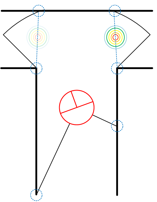
It is important to remark that the position of the detected openings is given in polar coordinates with respect to the origin in the center of the robot. Also it is important to note t to note here is that, LLFD can detect several openings at the same time.
Detection Algorithm
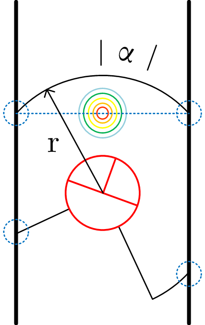
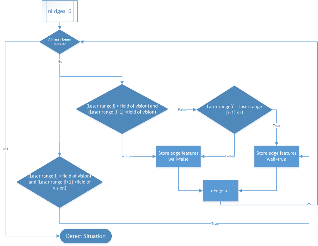
The LLDF uses a reduced field of vision in order to detect features of the environment. To be more explicit, a reduced field of vision means that the algorithm is only considering relevant information that is inside of a predefined range that is lower than the maximum range that the LFR can measure. The main idea is that with a reduced field of vision, it is possible to detect edges created by the objects that are intersecting the field of vision denote by the dashed circles as can be seen in the figure denoted by the blue dashed circles. The detected edges are stored in the next private variables declared in the class Detection variables
struct edge{
              bool wall; //flag that indicates in the edge detected is a wall or an open space
              double radius; //distance from the center of the robot to the detected edge
              double angle; //angle where the edge is located with respect to the referential frame of the robot
        };
edge edg[MAX_EDGES]; //array used to store edges
 int nEdges; //number of edges stored
Besides the function that is in charge of this detection is defined as
void extractFeatures( emc::LaserData& scan); //analyzes the raw laser data to detect edges in the field of vision
The figure shows a highly simplified flow diagram, where it is possible to appreciate the basic logic used in the function extractFeatures to detect the edges. Hence, it is clear to see that this algorithm detects a set of edges in each execution of the function. For this reason LLFD is executed continuously in the main loop during the operation of the robot.
The final step is to execute the function
void detectSituation();//uses de detected edges to define openings
Which uses the set of detected edges to define the openings in the surroundings of the robot. The main idea of this function is to analyses couples of consecutive edges that have the variable wall set as true and false respectively. For each pair of edges analyzed the next steps are executed:
- Find the Cartesian coordinates of the edges with respect to the robot frame.
- Find the distance between the edges.
- Find the Cartesian and polar coordinates of the middle point between the edges.
Therefore, the information obtained in the previous step permits to filter the possible openings using the next set of filters:
- Minimum angle between edges.
- Minimum distance between edges (opening width)
Besides this information, the algorithm also allows to detect special situations as open spaces, dead ends and safety limits.
(Mapping the Maze) Feature Detection
Special Situation Detection
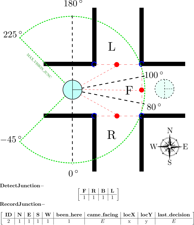
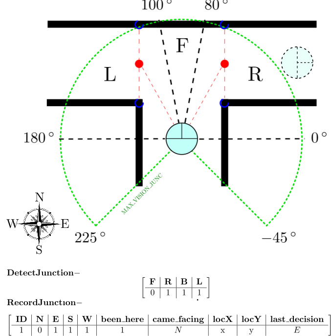
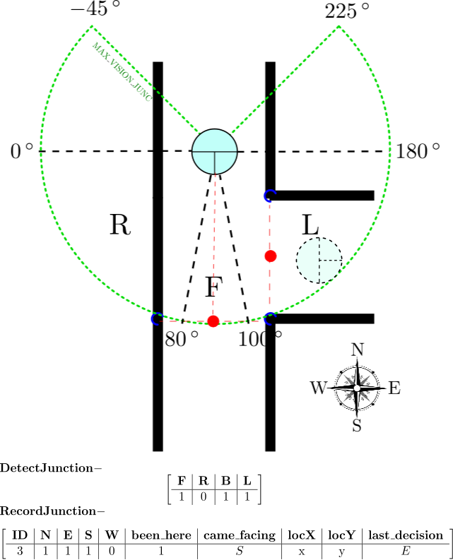
To detect special situations we use an extension of our low-level feature detection function which runs at an extended maximum laser range (MAX_VISION_JUNC). In this way, we are able to detect and identify the type of special situation before the decision has to be provided to the navigation algorithm. Having a longer range (not more than 0.5 meters more) provides enough time to send useful data for the solver to apply logic.
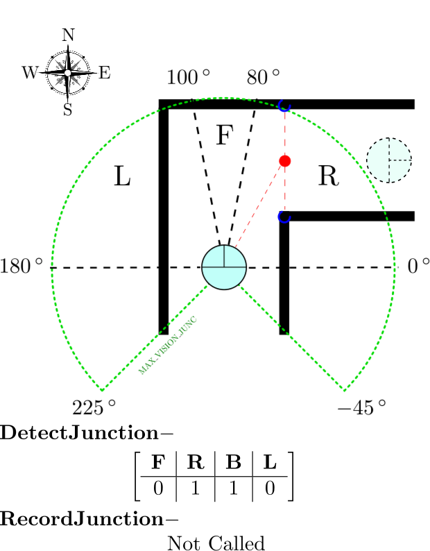
The algorithm works similarly in the way that it detects the number of openings that appear inside the range of vision and also calculates their angle in degrees with 0 degrees as presented in the figures. Inside the feature detection class there is a secondary loop that first checks the number of openings and provides information about what type of junction we are dealing with. The function then checks on which side of the robot the opening is located with the possible outputs being stored in an array - [math]\displaystyle{ \left[\begin{array}{c|c|c|c}F&R&B&L\end{array}\right] }[/math], standing for "Front","Right","Behind","Left". Inside that array, "1" stands for opening, while "0" stands for wall. To recognize those accordingly, we have separated the field in front of the robot in three different subparts depending on the angle from 0 degrees to the middle of the opening:
- [math]\displaystyle{ 0^{\circ}\quad \text{to}\quad 80^{\circ} }[/math] - The opening is on the Right of the robot
- [math]\displaystyle{ 80^{\circ}\quad \text{to}\quad 100^{\circ} }[/math] - The opening is in Front of the robot
- [math]\displaystyle{ 100^{\circ}\quad \text{to}\quad 180^{\circ} }[/math] - The opening is on the Left of the robot
Using this split, we make sure that the opening is detected and recognized soon enough while allowing room for heading error. The figures on the side of this text demonstrate the robot vision area and directional split. The red dots indicate the point in the middle of the opening as detected from the detection class. An important thing to notice is that the frame is body-fixed such that no matter what the heading of the robot is w.r.t. the global frame, the feature detection will provide adequate directions available. This is important for overall mapping. As can be also seen in the figures, we have added the functional outputs from the map entries as well. The reader is referred to the Maze Map section
A special algorithm was added inside the function to add more robustness to the feature detection. The algorithm stores a copy of the output of the system the moment it is initially calculated and then checks for each loop tick up to a pre-specified value whether the output remains the same, before outputting it safely to the global coordinator. In pseudo code, this looks like :
  if (no_opening_detected){                    \\ Wait till a junction is found and output nothing before
        return nothing;
    };

    else if (counter < robustness_value){        \\ Loop that checks whether we have received the same values

         if stored_output == current_output {    \\ If they are the same -> increment the counter
             counter += 1;
             stored_output = current_output;
         } else counter = 0;                     \\ If not -> reset the counter
    };

    else {                                       \\ Only output once the counter has reached the robust margin
        return output
    };
Note that the path the robot came from is always available and stored as "1" in the "Behind" array box. If only a corner is detected (1 opening) then it is treated as a simple situation, where no special decision has to be made and no map entry is needed, since the potential field navigation algorithm will always take that opening. However, a flag is still raised to notify the global robot positioning system and change the heading of the robot with respect to the global frame. Additional to those flags, quite a big part of the map entry for this special situation is also recorded the moment the openings are detected. An algorithm first checks the facing direction of the robot with respect to the global coordinate frame before he solves the situation and then compares with the number and location of openings it detected. Then each opening is recorded at the correct array entry of the map by converting the frames.
Door Detection based on vector projections
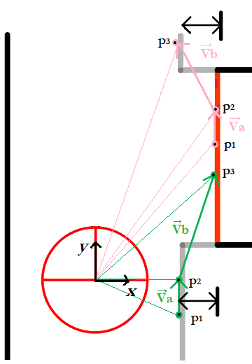
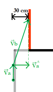
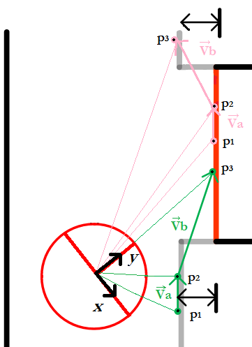
The door scanner algorithm was made such that is independent of the robot orientation (see Fig 2). For that purpose, a vector projection approach (see Fig1) was used in order to detect an indentation of approximately 30cm which could be a door.
The vector projection approach described in Figure 1 is applied to the full range of the LRF (270°). The 3 points, which define the start and end-points of the vectors, are chosen such that two points (p1 and p2) are relatively close (20 beams between each other) and aligned and the third one is a bit further (60 beams with respect to p2). In this way, we calculate 2 vectors: Va which defines the direction from p1 to p2 and the Vb which defines the direction from p2 to p3 (see Fig1). Once we have those 2 vectors, vector Vb is projected onto the perpendicular vector of Va, the resulting projection will be equal to the indentation of the door. When the robot finds a 30cm positive projection a door is marked (see Fig 3). Following the same approach the other side of the door will be found when a negative projection of 30 cm is found (see Fig4).
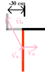
These projections will be stored in an array if and only if the projection is 30 cm plus a deviation of +- 10 cm. The corresponding door location will also be saved on another array such that we can calculate in a later stage where the door is located. The approximate door entrance/exit location will be defined by the middle beam with respect to the points p2 and p3.
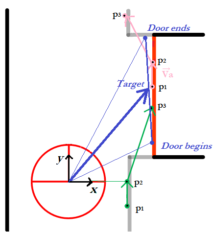
Once both arrays are filled (projection tracking array and door entrance/exit location array), we will find in which case does the projection data jump from having a positive projection (door entrance) to have a negative projection (door exit), which will define a door on the right. Note that when the door is on the left we will need to find projections from negative to positive. The door target will be set by calculating the middle beam of the entrance and exit beam location (see Fig 5). Once the target radius is relatively smaller than a certain DOOR_TRIGGER-value we consider that we are inside the door area, such that the global coordinator can execute the necessary algorithms, which contains amongst others sending a command to navigation that the robot needs to stop.
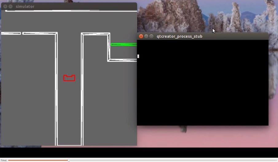
As this algorithm is designed to work within straight corridors it will be disconnected while turning in order to avoid false doors. However, on the last experiments, the algorithm was sometimes detection doors. Therefore, on the last moment for the maze competition we decided to use a door detection algorithm based on corridor width. A demostration of this algorithm running in s simulation can be found int the following video. The Doorscanner Class created which implements the door detection algorithm can be foudn here: Doorscanner-Class.Note that here the projected vector was defined on the opposite direction with respect to the figures.
Door Detection based on corridor width
This door detection algorithm keeps a track of the distance from the robot to the left wall and the right wall. The algorithm keeps track on two arrays of the wall limits on both sides. On every loops the a new wall limits are added while the oldest ones are removed, in this way the tracking array is always a 5 element array. Next both arrays are evaluated and when a change of 30 cm plus a deviation of +- 10 cm is detected, the door was found. This usually happpens once the robot reached the first corner of the door, however we wait until the robot is inside the door area to set the doorArea boolean variable to true. On the following video you can see a simulation were the aboved described algorithm is working. It can be observed that the robot does no give false door alarms when turning and that the robot stops inside the required door area.

The Doorscanner Class created which implements the door detection algorithm can be foudn here: Doorscanner-Class
(Mapping the Maze) Robot Position

The main function of the Global Robot Positioning System (GRPS) is to provide the location of Special Situations after visiting them and "predict" the location of Special Situations when encountering one. The Global Position of Special Situations is of great importance in building a topological maze map. This functionality was fully integrated in a robotPosition-class in the C++-language. This class mainly contains the following elements, a more detailed explanation/description is given after this short one:
   void robotPosition::initialDistance(emc::IO &io, emc::LaserData &scan);
     // This method determines the distance to the next perpendicular wall.
   void robotPosition::readyForCorner(emc::IO& io, emc::LaserData& scan);
     // This method executes all the functionality when a Special Situation is detected for the first time.
   bool robotPosition::Cornering(choices Direction, emc::IO& io, emc::LaserData& scan);
     // This method is active when the robot is turning and keeps track of the robot's position during it.
     // The choices Direction input specifies the direction we are turning to, Forward/Right/Back/Left
   void robotPosition::CorneringFinished(choices Direction);
     // This method  executes after a corner has been completed. It makes sure that the LandMark is updated as well as PICO's own position.
Some remarks about definitions: a special situation is defined as being a: corner (both to left and right), X-junction, T-junction, Dead-End, U-Turn. In the function-names above Cornering is being used, this method actually refers to turning of the robot it activates whenever the robot is changing orientation. Also throughout the next explanation the term LandMark will be used to indicate the representation of a Special Situation in the Maze Map. The global position of the robot will be represented by a (x,y)-coordinate where the (positive) x-direction is oriented along the East and the (positive) y-direction is oriented along the North.
Detailed Explanation/Description
Now we will give a more detailed explanation/description of the Global Robot Positioning System (GRPS)-class, this will be done using following the robot throughout a sample maze presented in the picture to the left. Also the execution of the different methods in the RobotPosition-class is presented in the FlowChart to the right. The following functionality is executed during its execution
Position 1: The Robot is initialized at Position 1 where first the initialDistance-method determines the distance from Position 1 to the perpendicular wall in front of the robot which is denoted by A. We store this distance in StoredDistance. The Robot then starts driving, at some point it will reach
Position 2: The method readyForCorner-method will be triggered by the detection of a Special Situation. At this point the distance from Position 2 to the perpendicular wall (A) in front of the robot is determined and stored in LeftInCorridor. Knowing the orientation of the robot (which is North when starting by definition) we can find the current position of PICO by adding the distance
to the y-coordinate. E.g.: the robot starts at (0,0) facing North, if then StoredDistance = 5 [m] and after arriving at Position 2, we find LeftInCorridor = 1 [m], we know that Position 2 is located at (0,4) with PICO (still) facing North. As the distance from the mid-point of the Special Situation (which will be the Global Position stored in the LandMark) to the point where the Special Situation is detected Position 2 is quite constant we can now estimate the Global Position of the LandMark. (This is also represented at Position 6) E.g.: using the previous example and the fact that the distance from the mid-point of the Special Situation to the point where the Special Situation is detected is 1 [m], we estimate that the LandMark is at (0,5). Aside from estimating the global position of the LandMark, the readyForCorner-method also stores the odometry data in StoredOdometry of the robot at Position 2 is stored in method, the General Coordinator then starts the execution the Cornering at the Special Situation. Position 3: During turning the CurrentOdometry is compared to the StoredOdometry in the Cornering-method, if the orientation of the robot changed 90 degrees in the correct direction (turning left or right) the distance from Position 3 to the perpendicular wall (B) in front of the robot is determined and stored in StoredDistance. When the General Coordinator recognizes that the Special Situation has ended the CorneringFinished-method is ran. This method adds the difference
to the global position of the PICO robot. Also the position of the LandMark will be determined more precise (hence not an estimate anymore): in this case the x-coordinate determined before turning (Position 2) and the y-coordinate after turning (Position 3) will be used to form the global position of the LandMark will be stored in the Map. E.g.: using the previous examples and the fact that the difference [math]\displaystyle{ CurrentOdometry-StoredOdometry }[/math] is 1.5 [m] in both directions the LandMark position which will be saved will be (0,4+1.5) = (0,5.5).
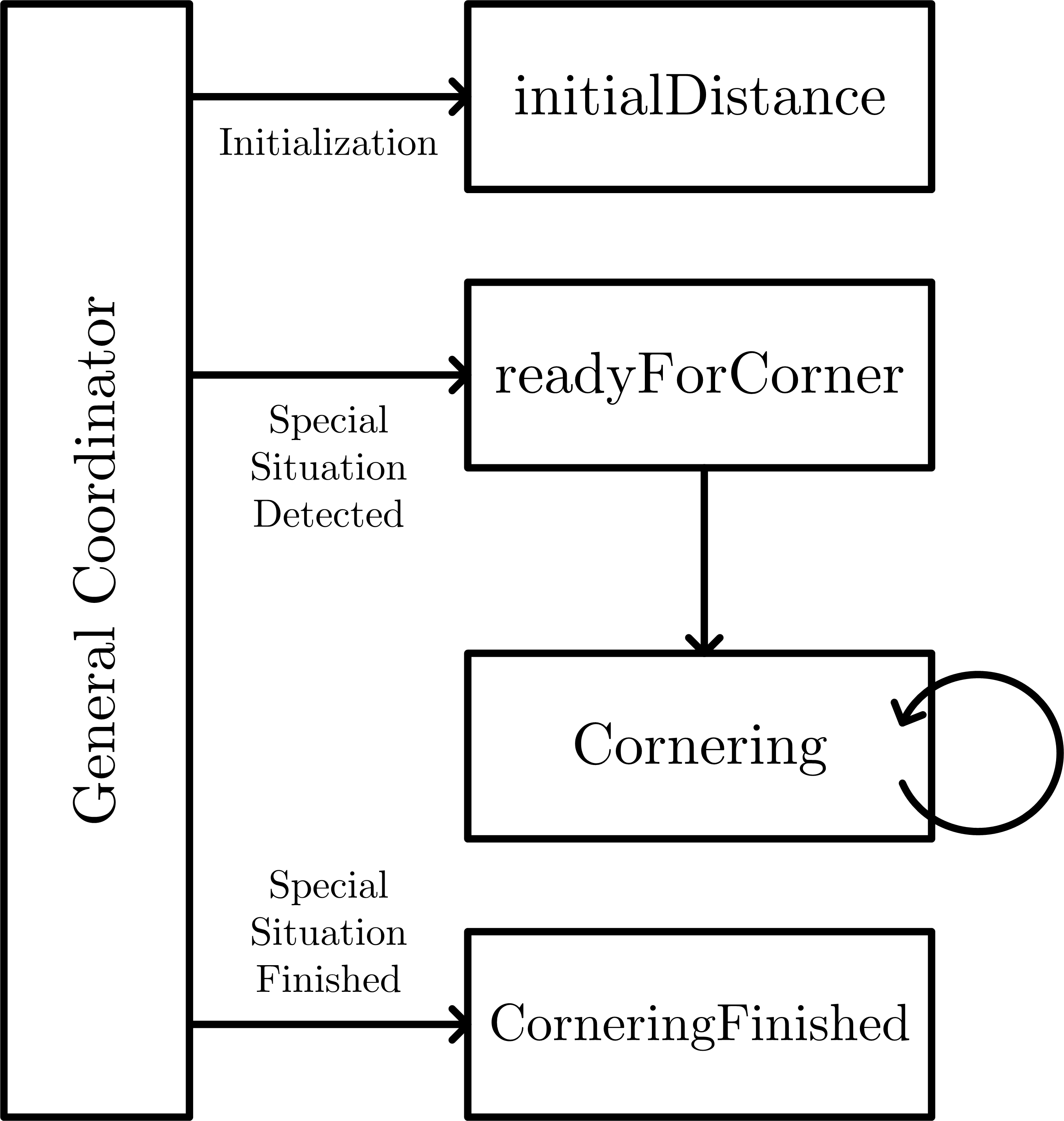
- Once the robot detects the Special Situation of Wall b the algorithms executes from step 2 above. Note that after this first turn the orientation of the robot has changed, note that the distance [math]\displaystyle{ StoredDistance-LeftInCorridor, }[/math] will now be added to the x-coordinate. This change in orientation will also be applied to the estimate of the LandMark-position in step 3. This describes the algorithm when the robot changes orientation, note that there are three special cases: U-Turns (Position 4), Dead-Ends (Position 5) and Straight-On-Junction (Position 6), these will be explained below
Position 4: On approaching a U-Turn we can not yet detect whether it is a U-Turn, therefore the U-Turn algorithm starts when the Cornering-method recognizes a U-Turn because the robot turned more than 135 degrees and the General Coordinator still didn't signal the end of the Special Situation. At the moment of detecting the U-Turn the measurement of the distance to the next perpendicular wall, which was taken when the robot turned 90 degrees, is discarded. A new measurement is made when the robot turned 180 degrees and then when the General Coordinator signals that the Special Situation is finished, the CorneringFinished-method is ran.
Position 5: On approaching a Dead-End we know that the it is a dead-end (or a door), the Door Algorithms executes. After waiting some time we either have to turn around, the General Coordinator signals a 180-turn. The same algorithm as for turning is used but know making the measurement at 180 degrees and of course changing the orientation differently.
Position 6: It can also happen that we approach a T-(or X-)junction where we will go straight, in that case the junction has to be mapped anyway, in that case the estimate of the LandMark from the readyForCorner-method will be used. Then because we are driving straight the Cornering-method will not be triggered. Note that in this case we will not improve the location of the LandMark position as we do not turn on that junction.
Demonstration of Algorithm
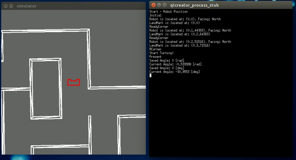
For a demonstration of the Global Robot Positioning System, click on the picture to the left. This will open a Youtube-Video (GRPS Demonstration) with a demonstration of the algorithm described above. To show the processing of the algorithm most clearly this test uses the teleoperation-tool for the simulator to drive PICO around, via the Qt-Creator terminal the Stimuli, normally provided by the General Coordinator, are provided by the user. The following commands are used:
- Initial: runs the 'initialDistance-method.
- ReadyCorner: runs the readyForCorner-method.
- LCorner: runs the readyForCorner-method with Direction left
- RCorner: runs the readyForCorner-method with Direction right
- DeadEnd: runs the readyForCorner-method with Direction back
- SpecSitFinished: runs the CorneringFinished-method.
- Present: presents the current angle and the saved angle from Odometry, this is used to position the robots in these simulations.
During the video constantly the Current LandMark and Robot Position are updated and printed in the Terminal interesting to see is the LandMark Position of the second junction encountered:
- Before the Loop the Junction is placed at: (0,3.53)
- After the Loop the Junction is found to be at: (-0.03,3.38), which is off 3 cm in x-direction and about 15 in y-direction
Note that in the video around 5.14 (min) that the algorithm is when coordinator doesn't give the right commands and the robot is moved when the correct methods aren't active, note however that this would have a severe effect on the Global Position of the robot if it was moved during this period.
The code of the methods explained here and the class definition of the GRPS is presented on robotPosition-Class
Maze Map
In our design we decided to build a semantic map using a topological tree structure. To achieve this, we store each special situation in the maze in an array structure with unique identifiers and characteristics. The array entry for a single special situation has the following information inside it :

where :
- ID - unique number of the map entry.
- N - Entity in the north part of the junction.
- E - Entity in the east part of the junction.
- S - Entity in the south part of the junction.
- W - Entity in the west part of the junction.
- All of the above four are with respect to the fixed, global coordinate frame.
- Possible states are 0 for wall, 1 for opening.
- been_here - Marker that shows whether this situation has already been encountered.
- Possible states are 0 for never been here, 1 for been here once and 2 for been here twice.
- came_facing - Direction the robot came from. Again with respect to the fixed global coordinate frame.
- locX - Coordinates in 'x' as received from the GRPS
- locY - Coordinates in 'y' as received from the GRPS
- last_decision - Last decision made at this junction with respect to previously in the array stated characteristic of the situation.
With this method, all important information about the maze is stored and a semantic map of the maze can be built as all the data is available at all times inside the mapping class, where the solver logic has access. Most of the information about each special situation is recorded initially when the DetectJunc function detects one. Inside that function, each opening detected is checked with respect to the robot's current heading and the openings are classified and stored at their accurate location in the array. Also a flag is raised for the solver if the junction has already been recorded before to help with algorithm adaptation.
The rest of the information about the junction is recorded after the situation is resolved and a decision is already made from the solver. A function called RecordJunction reads the decision made by the solver, which is in the form [math]\displaystyle{ \left[\begin{array}{c|c|c|c}F&R&B&L\end{array}\right] }[/math]. Then depending on the direction taken, the current heading of the robot is recalculated with respect to the global frame by the following function, where the numbers 1, 2, 3, 4 denote North, East, South, West respectively :
// Forward drive (N)
    if (decision.F == 1){
        facing = facing;
    }
    // Clockwise turn (E)
    if (decision.R == 1){
        facing += 1;
    };
    // Anticlockwise turn (W)
    if (decision.L == 1){
        facing -= 1;
    };
    // 180 turn (S)
    if (decision.B == 1){
        facing += 2;
    };
    // Recalibration
    if (facing < 1) {
        facing = 4;
    }
    if (facing > 4) {
        facing = 1;
    }
Note that the initial heading and global frame assignment are done at the beginning with North being PICO's starting direction. Finally the rest of the array is filled up - coordinates of the junction from the GRPS, decision which was just made and the value of been_here being incremented to make sure next time this junction is reached a different decision will be taken to avoid loops. The reader is referred to check Special Situation Detection section for figures which demonstrate maze map entries after a decision is made at various type of junctions.
In this section, the design and development of the Robot Navigation for the A-maze-ing Challenge is presented. Robot Navigation is divided in three main blocks:
- Path Planning: real time path planning. Implementation of Potential Field method.
- Robot Drive: low-level control of omniwheels. Only block with low-level connection with actuators.
- Navigation coordinator: high level function of Robot Navigation. This functions communicates with Global Coordinator and coordinates the tasks inside Robot Navigation.
The different blocks will be presented in detail in the following sections.
Path Planning: Potential Field
Mobile robot path planning is typically stated as getting from one place to another. The robot must successfully navigate around obstacles to the target point and do it efficiently. In the A-maze-ing Challeng we have to find the exit of a maze, trying to find the shortest path and not colliding with obstacles. Therefore, Path Planning is one of the most critical tasks.
In order to choose which appropriate method to use, the state of the art of robot navigation was studied. During this analysis, methods using Potential Field, Kalman Filter or Hugh transform were considered. The variables analyzed were complexity of implementation, accuracy of the method and previous work. After this initial study, Potential Field method to calculate robot path was used. Potential Field resulted easy to implement and widely extended. Potential Field method has a known number of limitations (e.g. local minima), nevertheless its “straight forward” implementation was considered as a great asset due to the characteristics of this challenge.
Introduction to Potential Fields
A potential field is a reactive architecture as it reacts to the environment. The potential field method treats the robot as a point under the influence of an artificial potential field. The goal acts as an attractive force on the robot and the obstacles act as repulsive forces. So by combining these two parts a virtual force is induced that moves the robot towards goal and keeps it away from obstacles. While potential field planners follow the gradient descent of the field to the goal they always find the shortest path from every possible start point. An example of the different fields can be seen in the next figure. The equations which describe this method can be found easily online. More related information about this method can be found in [NAV-1].
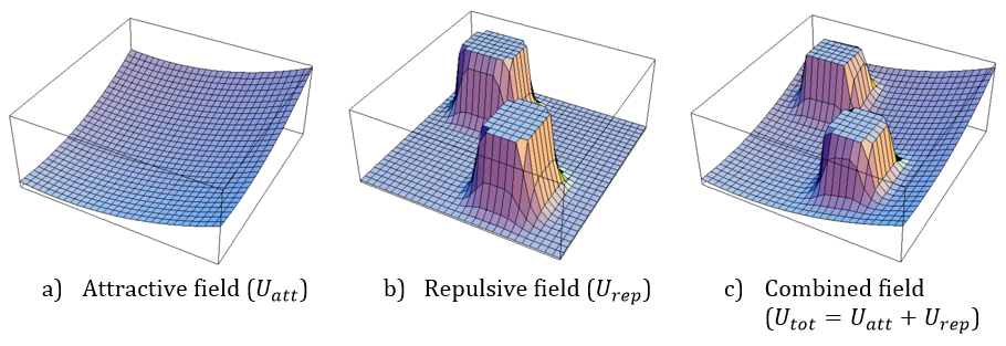
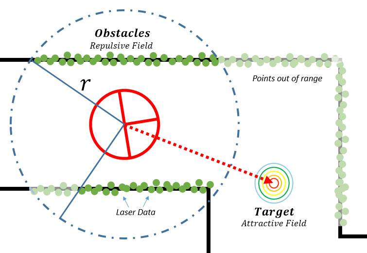
Potential Field method can be implemented offline, when complete information of a map or an environment is known or can be generated using real-time sensor data. In our implementation we are generating potential fields using the real-time sensor data, i.e. using Laser Range Finder (LRF) data. In our approach, LRF data is used to compute the obstacles: all points from LRF that are inside a fixed range (R, configurable) are considered obstacles.
On the other hand, the target (attractive force) is estimated in two different ways: a) using a fixed target in the center of the robot, or b) selecting an opening which has been calculated by “Low-level feature detection” function. The first option (a) will be used in case of not detecting any openings. When more than one opening is detected (e.g. “T” Junction), Global Coordinator must send the desired next movement (front, turn right, etc.) to Robot Navigation (i.e. Navigation Coordinator).
Robot Drive
The only function which can have direct access to the actuators (omniwheels) is Robot Drive. With this division, the high and low level functions of Robot Navigation are decoupled. In general words, this function receives the direction of movement and sends the command to move the omniwheels of PICO.
Furthermore, this function checks the maximum velocity of the bot, as well as to have a “progressive acceleration”. Also, this function controls the velocity while turning to increase safety. A simplified flow diagram can be seen in the next figure.
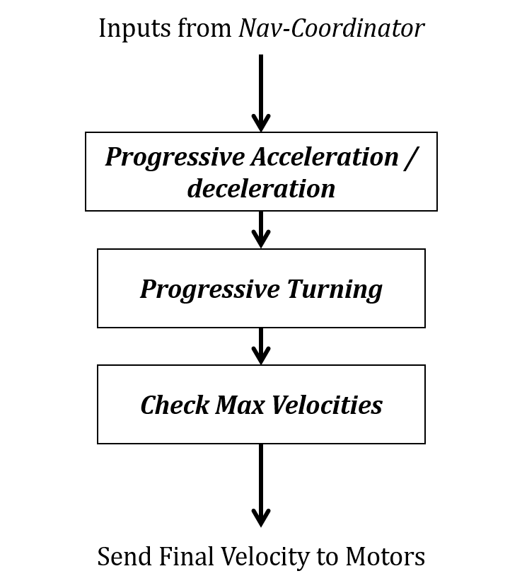
In order to keep the software design decoupled, a Navigation Coordinator block is used. Using this block, the functionality of Robot Navigation is divided between coordination tasks (FSM) and its low and high level functionalities (i.e. “Drive” and “Potential Fields”). Navigation Coordinator is in charge of receiving commands from Global Coordinator and enable and disable the different skills of Robot Navigation.
The different commands that Navigation Coordinator can receive are:
- Simple movements: Right, Left and Forward.
- Decisions: choose the most adequate angle to make a simple movement (RGT, LFT or FWD).
- Door sequence: sequence to open the door and cross it.
- Turn 180 degrees: in case of dead end.
- Safety condition: when safety condition is triggered.
- Emergency condition: stop in case of emergency.
Demonstration of Algorithm
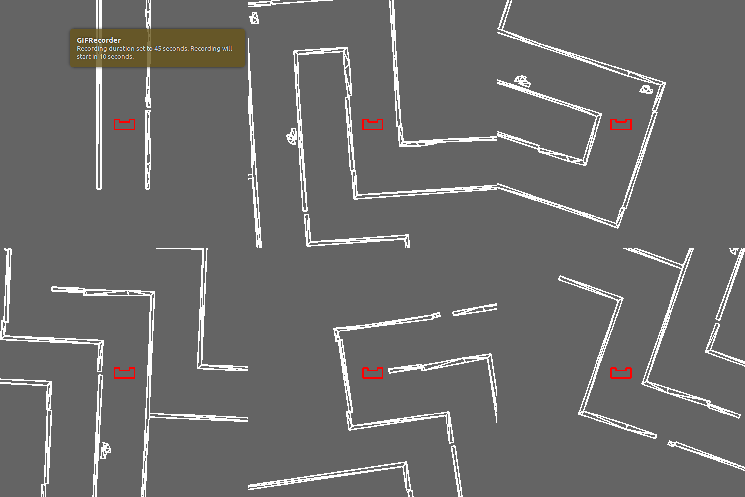
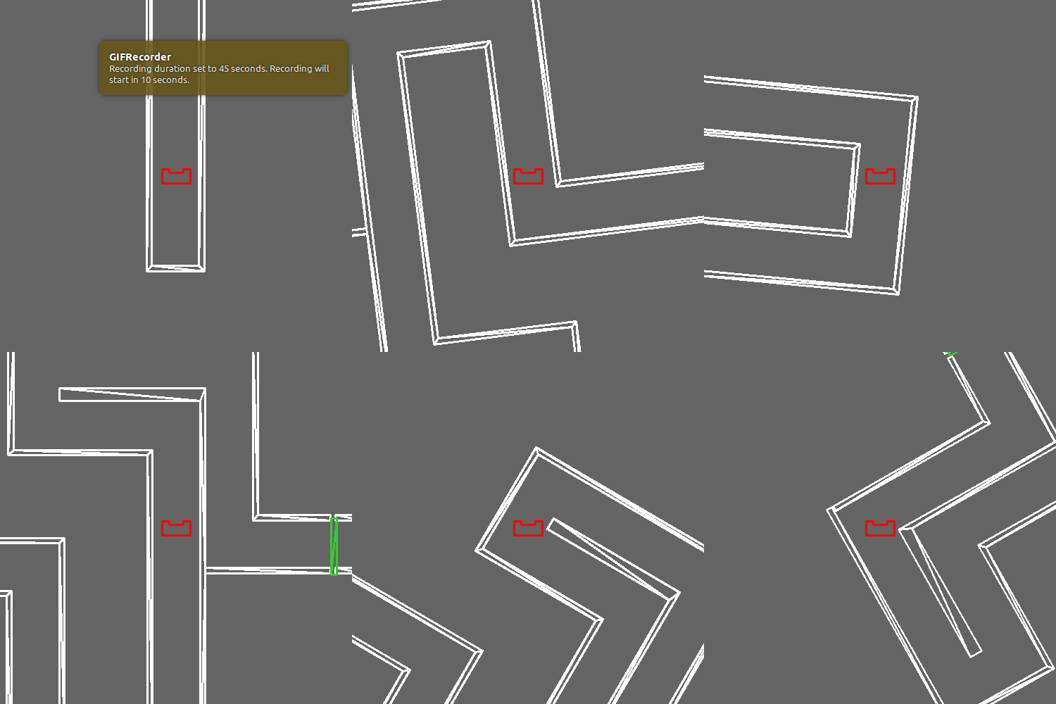
The implemented navigation method is presented in the next animated gif. In the following examples, two different mazes are used: realistic maze with average width of 1 m (LEFT) and a regular maze with a constant width of 0.70 m (RIGHT). In these two examples, path planning based on Potential Field is used. The target of the Potential Field is updated using the detected opening (Low-Level Feature Detection). Moreover, progressive velocity during acceleration and turning (presented in subsection Robot Drive) are applied. In the simulation can be seen that the robot drives quite smoothly in both cases, reaching maximum speed when going straight and decreasing speed while turning, with realistic and narrow scenarios.
|
|
Code & Composition Pattern
Arrived to this point, it is important to comment the code structure of Navigation class. During the completion of this challenge, great efforts were made in order to apply the Composition Pattern to the software design. Due to the fact that several people must have access to the same code and that the different classes must be easy to integrate made the decoupling highly important.
During the development of the code, we notice that Navigation class was (probably) the most important class (being needed for other teams to test full functionalities). One key decision was to put noticeable effort during the definition of the interfaces (between modules, e.g. Global Coordinator - Navigation) and defining internal functionalities, highlighting the importance of decoupling. The different priorities for the skills (which skill shall be implemented first) were also defined at this step. Thanks to the decoupling, all teams could work in parallel and were able to test their individual contributions without waiting for the final version of Navigation.
Returning to the Composition Pattern, the implemented modules inside the Navigation Class container are: Configurator, Functional Computation, Coordinator, Monitor and Logger. Not all modules were considered (scheduler or composer) due to the characteristics of the challenge (we considered the implementation of these modules too complex for the needs of the challenge). For some modules, the Composition Pattern can be seen explicitly in the code (e.g. different function), while for other ones its relation is implicit in the software. The different modules are briefly introduced below.
- Configurator: the configurator module is able to configure all parameters related to Navigation, e.g. maximum values of velocity, acceleration or safety limits, weights for Potential Field, etc. Mostly the Configurator functionality has been implemented in the constructor of the class and using the file "parameters.h". When constructor is called, it initializes the local parameters (local to the class) using the values stored in "parameters.h". Therefore, to configure the system (e.g. while tuning the weights for Potential Field), only the values of the parameters have to be modified. Also, we considered the use of different "parameters.h" files with different configurations (e.g. safety or fast). We assumed that the configuration values are known in advance and it's not necessary to change them during run-time.
- Coordinator: the coordinator is explicitly implemented in Navigation-Coordinator. Navigation-Coordinator can send commands to the Functional Computation modules, enabling/disabling specific skills. Some of the commands are drive forward, turn right/left, request open a door, etc. It can also select which Path Planning method is used (e.g. receiving the orientation of the target from Low Level Feature Detection, or generating a target in the center of PICO).
- Functional Computation: two different modules are purely for functional computation, i.e. Potential Field and Drive. Drive is in charge of the low-level movement of the bot, i.e. Move X/Y/thetha. On the other hand, Potential Field estimate the potential fields and returns the desired path direction.
- Monitor: the monitor is implemented implicitly in the code. We conceived the monitor as the module in charge of checking the minimum distance, keeping track of time, etc. Its functionality is divided internally in the Navigation code. E.g. Navigation-Coordinator checks if the flag of minimum distance has been triggered or if there is any emergency status.
- Logger: during the execution of the tests, various (self-made) loggers were used. These loggers were extremely valuable to analyse and understand the behaviour of PICO in "real" environments.
Finally, a simplified version of the class is presented in the following link: Navigation, simplified code.
In order to simply the code, several lines have been omitted, trying to highlight its relation with the Composition Pattern (and how we conceived it).
Conclusion
The Potential Field algorithms are popular due to their simplicity and easy implementation. For simple scenarios, it gives satisfactory results.
Nevertheless, the Potential Field method has several disadvantages or limitations:
- The local minima problem: new vector with zero magnitude is calculated. As a result the robot remains motionless.
- Another drawback is that, the robot cannot pass among two closely spaced obstacles
- While moving in narrow passages the robot is effected by repulsive forces, which causes unstable movement of the robot.
Various of these limitations were experienced during the implementation of the algorithm. We observed that this algorithm (i.e. its related parameters like the weight of the target or the radius of the potential field) is extremely affected by the environment. One example is that the performance and behaviour of the bot varies with the configuration of the maze (highly affected in narrow corridors, as mentioned before). Therefore, a configuration/calibration of the different parameters is needed to ensure desired performance. The previous problem is really inconvenient in the case of the A-maze-ing Challeng, when you want to have a robust navigation with very limited test hours.
To sum up, we can conclude that the choice of Potential Field for navigation was a good decision due to the characteristics of the challenge. This method was implemented quickly with good performance. It allowed us to focus our resources in other levels of the code. Nevertheless, the limitations of the algorithm affected during test and its behaviour is not predictable. Therefore, we consider that an extended version Potential Field or more advanced navigation methods are needed for more complex scenarios. Due to the division of the code using a Composition Pattern, the Navigation class can be easily modified in order to include other navigation methods (thanks to the decoupling).
Solving the Maze
To solve the maze we decide to use an algorith that always look on all the possible solutions and based on the information given by Maze Map, take the decision.
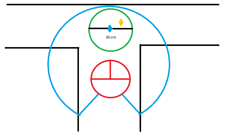
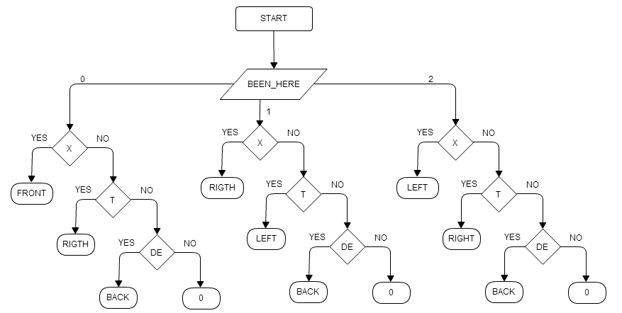
The program will recognize between three different situations, the first situation is when there is not previous information and the system needs to recognize between “X-Junction”, “T-Junction” a “Dead-End“. Based on this recognition the system will take the decision, here three cases are considered based on the knowledge that the robot can approach to the same point more than once. If this happend a different decision is made based on the number of times that the system approach to a junction. The next diagram shows how the algorithm works based on a case function. It is important to note that the cases for been_here can be 0, 1 or 2 and this means that the function will check in Maze Map if the coordinates for this possition had been reached before with a range of 30cm. appart from the coordinates obtain when the function is called. If the coordinates are inside this range the system will recognize the function as been here and if some other coordinates are also in the same range the system will recognize it also, based on this the number of times of been_here can be stablish and depend on this an specific logic will be follow.
In the case that the system is called because a possible door is reached the system will corroborate the recognition of the door, in case of a positive response the system will check if the door is open and if this happend the system will choose always to take the corridor of the door open. The logic of this function is represented in the diagram below.
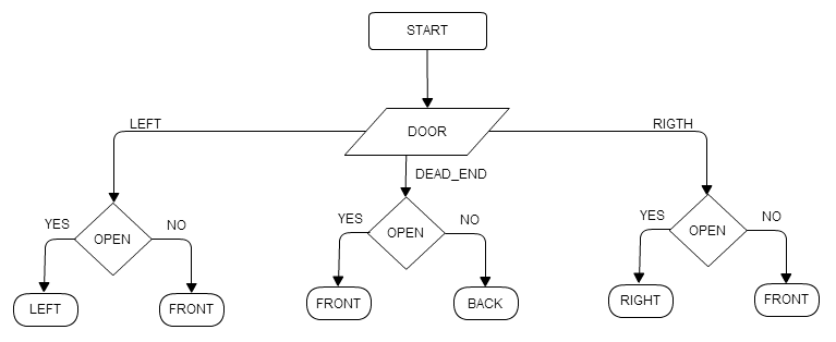
With this algorithm we are able to avoid loops and to get an stablish preference to always take the door when this is find it.
Global Coordinator
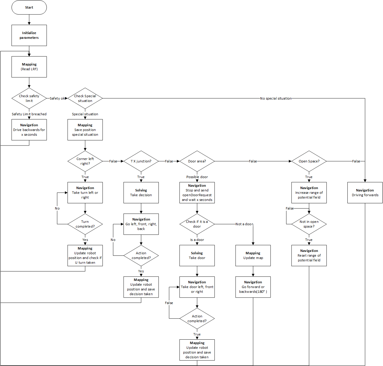
The working of the General Coordinator is described in the flowchart given in the figure on the left.
First, the robot is initializing his parameters. Also the robots position is initialized. Then, the robot is reading the Laser Range Finder (LRF) data, which is first checked on safety. If the robot is too close to a wall, the safety limit is breached and the robot moves backwards for 2 seconds before it continues with solving the maze.
If safety is not breached, the robot is driving forward until a ‘Special situation’ occurs. A special situation is defined as a corner, T- or X-junction, a possible door and an open space. If a corner occurs, the navigation of the robot makes the turn. When the turn is completed, the robot first checks if the corner was a U-turn. Then, the mapping updates the world map and the global position and the facing, e.g. north, west, south, east, of the robot.
Another option is that there is a T- or X-junction. In this case, the solving algorithm is used to determined which path to take. After the decision is made, the robot completes the action. The mapping updates the world map and robot positioning afterwords to keep track of all paths taken.
It is also possible that a dead-end or a possible door in a straight corridor occurs. For both situations, the possible door has to be checked. Therefore, the robot has to stop and send an acoustic signal to request the door to open. Finally, after waiting for 7 seconds after the request is send, the door can be evaluated. If the possible door opens, the robot has to go through the door and update his mapping. If the door stays closed, mapping is done to prevent checking the door twice. Then, the robot continues forward for a possible door in a straight corridor. If the closed door was in a dead end, the robot rotates 180 degrees and continues forward.
The last situation is the open space. For the open space situation, the range of the LRF is increased to detect walls at every moment. Then, the target of the potential field can also be set and navigation can still perform his actions. When the open space is completed, the range is reset to his original value.
Maze Challenge
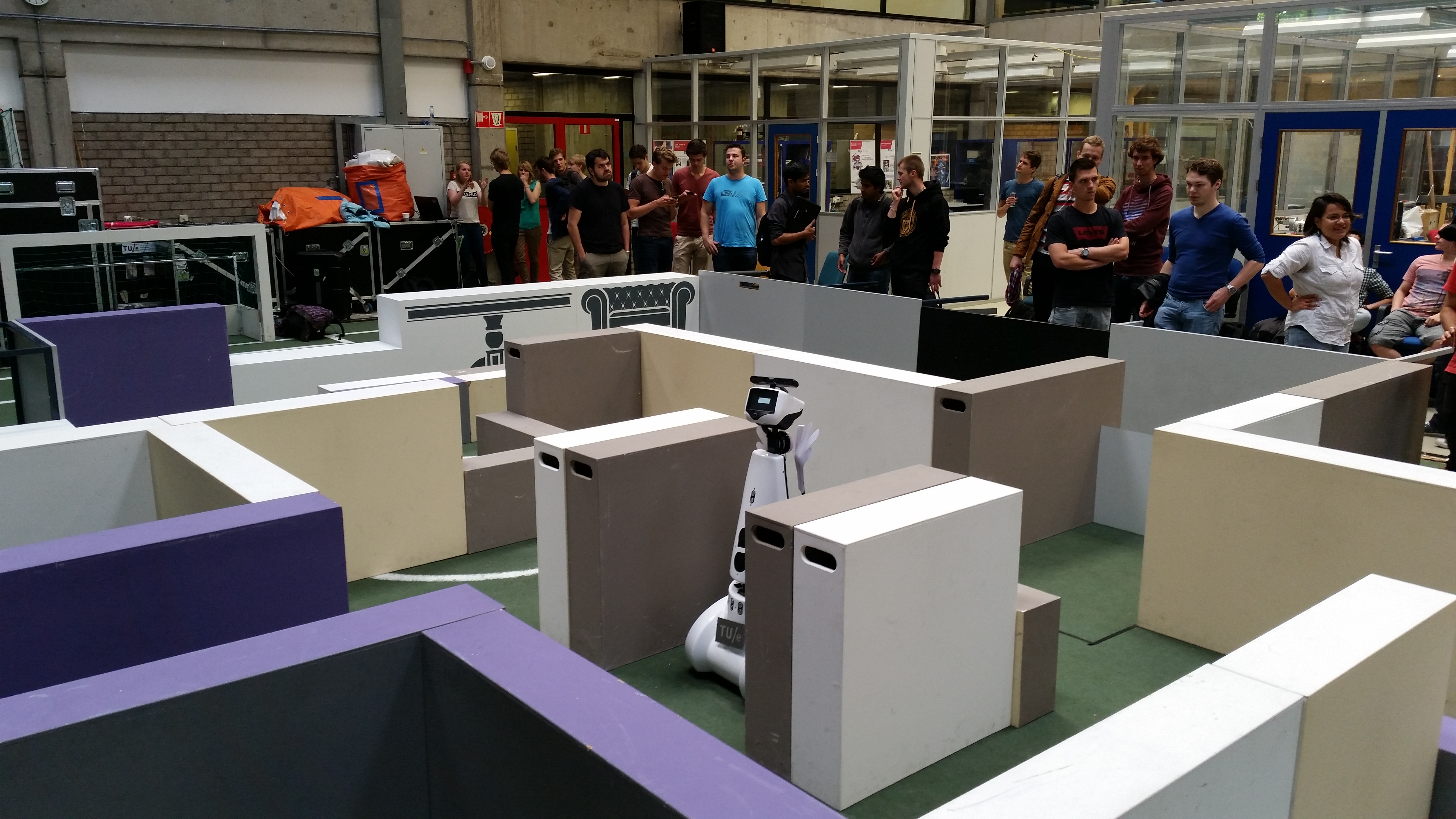
On the 17th of June 2015 the Maze Challenge was scheduled. The maze which has to be solved is shown in the pictures below.
 |
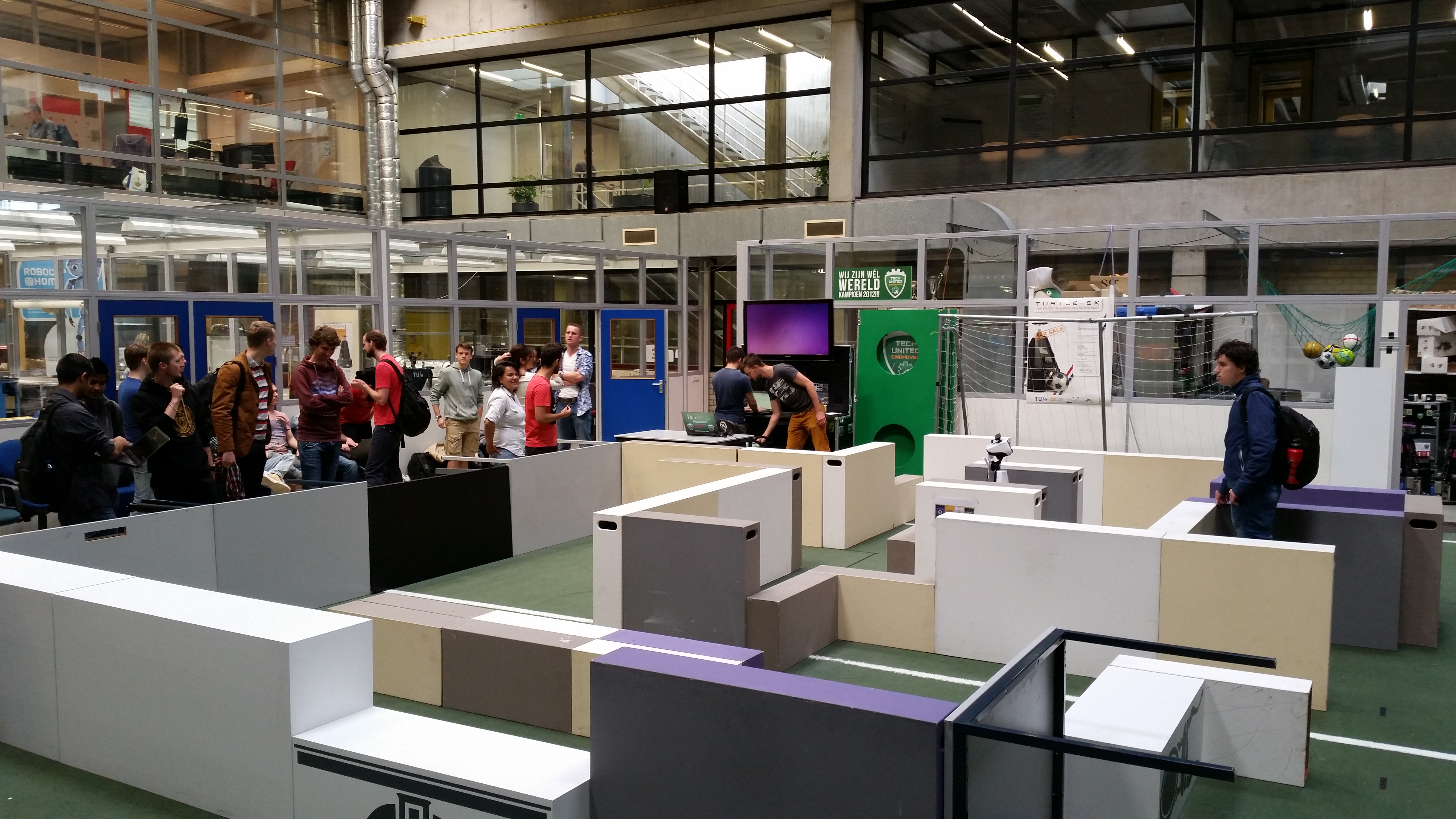 |
Videos of our both attempts to reach the end of the maze can be viewed by clicking on the two pictures below
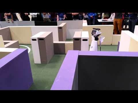 |
 |
Analysis First Try
- The code we used was adjusted at many places without testing. Therefore, the robot made wrong decisions at some points. In the beginning the robot already had a collision with a wall. But after the collision, the safety algorithm made the robot to drive backwards and continue the maze challenge. Then, at the T-junction with the door, the robot chose to go forward, which was also implemented in our algorithm of the solving. Then, when the robot did the T-junction for the second time, the dead end was not recognized and therefore, a possible door was not checked.
Analysis Second Try
- For the second try, the code of the test time, the day before, is used. As there were some bugs in there, the robot was not able to take the turn and proceed to the open space. Therefore, the robot was making loops. At the X-junction, the potential field placed the target at the wrong point which leaded to a turn of 360 degrees.
- In the end, our team thinks that the code of our first trial was able to perform the maze challenge successfully when the door is open. Unfortunately, during the maze challenge, we chose for the safe version.
Conclusions & Lessons Learned
Here we will summarize our Conclusions and the Lessons we have learned:
- Decoupling is Important!: we reckon it impossible to work with 7 people on one piece of software which is not properly decoupled. We think the time we spend in carefully designing the software as decoupled as possible is very valuable and allowed us to work more efficiently.
- Coordination at Different Levels!: in the actual software one General Coordinator is controlling almost the full software (except for Navigation, where there is the Potential Field Coordinator). Whereas in the Composition Pattern-presentation we presented that we would also have a Mapping Coordinator (read: Mapping Functional Composite Entity with Mapping Coordinator); this one was, due to lack of time, not implemented. Looking back we think that if we would have implemented this coordinator earlier the software of the General Coordinator would be more easy, which would also greatly improve the structure of the total software.
- Start Easy!: we think that we started to early on programming high-level functionality (solving algorithms, Global Robot Positioning System,...) while low-level functionality (navigation, low-level feature detection,...) were not working robustly enough.
- GIT is Inevitable!: as nobody of us knew how to work with GIT we used Dropbox throughout a large part of the project. In the end Dropbox however gave problems when suddenly many versions of differently algorithms were published in a high pace. Spend time in getting to know how to work with GIT in software-projects of this size it is Inevitable!
- Make most efficient use of Time-Limited Resources!: we learned that for example test time on the PICO robot is extremely valuable, use this as efficient as possible; we have learned a lot in this area. We also experienced the meetings with our Tutor as extremely valuable. We have taken great care to make sure these Tutor-meetings were as effective possible: getting feedback, presenting new ideas and discussing them; we have made sure (using agenda's and minutes) that before each meeting we knew what we had to discuss.
- Step Back and Get Overview!: in the end we think that we should have taken a step back more often; take a step back, look at the full project again and then look at the things you are doing. Maybe in some points we have stared blind on some pieces of software trying to get them to work while the concept might not have been the best to use.
- Leadership is Required!: to make sure Team-meetings and Tutor-meetings are planned (agendas, location, notes, presentations) one person has to execute these tasks, reserve time for this as these meetings are valuable.
- Embedded Motion Control: we have all experienced the course as being "one-of-a-kind" within the department of Mechanical Engineering and as extremely useful and interesting. The course not only increases your knowledge about programming of Robotic Systems itself but also on how to work in teams on one piece of Software. It is a lot of work (more than what is "advertised") but you'll get for that a lot of interesting concepts and definitely a lot of fun!
References & Material Used
During the course a large amount of material was consulted apart from the lecture slides:
Composition Pattern
- Bruyninckx, H. (2010). Task specification, control and estimation. Paris: Departement of Mechanical Engineering.
- Bruyninckx, H. (2015). Coding with the Composition Pattern. Eindhoven: Eindhoven University of Technology.
- Bruyninckx, H. (2015). Software for Complex Robotics Systems. Eindhoven: Eindhoven University of Technology.
- Vanthienen, D., Klotzbücher, M., & Bruyninckx, H. (2014). The 5C-based architectural Composition Pattern: lessons learned from re-developing the iTaSC framework for constraint-based robot programming. Journal of Software Engineering for Robotics.
Robot Functionality
- All documents that go with the course AMRx: Autonomous Mobile Robots on edx.org of ETH Zürich especially the textbook Autonomous Mobile Robotics which can be found in the course material.
- [NAV-1] Khatib, O., "Real-time obstacle avoidance for manipulators and mobile robots," Robotics and Automation. Proceedings. 1985 IEEE International Conference on, vol.2, no., pp.500,505, Mar 1985
- [NAV-2] Howie Choset, “Robotic Motion Planning: Potential Functions”, Robotics Institute 16-735, with slides from Ji Yeong Lee, G.D. Hager and Z. Dodds
GIT
- A very useful cheat sheet, summarizing the most important GIT functions can be found at GIT-Tower.