Mobile Robot Control 2024 Ultron:Final Report

(Group deadline: 21:00 28 June)

Introduction

High-Level System Description

（Yidan)

System Architecture

State Flow

(Liz)

Data Flow

The data flow diagram illustrates the interactions between input sources, processing modules, and output commands for the robots. There are three major input sources: the laser and odometry come from the robot sensors, and the map is uploaded by the user. The map provides the existing representation of the restaurant environment, including the table positions and order information. The laser detects obstacles in the environment. The odometry supplies information regarding the robot’s position and velocity.

The Localization module first receives the data from all three inputs to determine the robot's position relative to the map. Over time, the robot's theoretical and actual positions will eventually diverge because of accumulated errors from odometry conversions between theoretical and real movement. Therefore, it’s fundamental to ensure that the robot knows its exact position within the environment during its movement for accurate navigation. The position is then forward to both Global Navigation and Local Navigation modules.

Global Navigation uses the map to plan an optimal path from the robot’s current position to the destination through the combination of PRM and A* algorithms and updates the current target point for Local Navigation. Local Navigation uses the current position, the target point, and the laser data to adjust the robot's path dynamically, avoiding obstacles and navigating through tight spaces. It provides control commands for linear and angle velocity to guide the robot's motion.

The Stuck Detection module handles abnormal status during the local navigation. If the robot is within 0.2 meters of an obstacle according to laser data or cannot find a path to reach its target points due to an unknown static obstacle or being stuck in a local minimum, the stuck detection module is triggered. It stopped the robot and initiated a path re-planning through the Global Navigation module.

The process involves a continuous feedback loop, constantly monitoring and adjusting the robot's movements based on inputs and environments to ensure safe and efficient navigation towards its destination.

System components

Initialization

(Lu)

Localization

（Aori）

Global Navigation

（Yidan, Hao）

A* search algorithm

The A* algorithm we implemented has two working modes: it can build a planner by obtaining connected nodes from the grid information or the PRM algorithm. Since the grid information of the map is not given in the final challenge, we use the sampling nodes and connections between nodes given by the PRM algorithm.

In the main program, the A* algorithm is called before the while loop and after the PRM call. By adding reasonable conditional judgments and printing content, we ensure that the nodes and connection content can be read from the generated PRM image results. In order to deal with the situation where the node connection generated by a certain call to the PRM algorithm is unreasonable due to improper PRM parameters and the randomness of PRM, and then A* has no solution output, we set the corresponding judgment conditions. In this case, PRM and A* are called again. Ensure that there is an executable node list in the final pass to the local navigator.

Local Navigation

Dynamic Window Approach

Given a target point by global navigation algorithm and positions of obstacle by laser sensor, local navigation aims to calculate an available path to avoid collision with the obstacles as well as to move towards the target point. The outputs of all local navigation algorithms shown in lectures are directly the desired velocities [math]\displaystyle{ (v, \omega) }[/math] ([math]\displaystyle{ v }[/math] is linear and [math]\displaystyle{ \omega }[/math] is angular velocity) of the robot. There is no need to perform a path following task.

In exercising, we implemented both Artificial Potential Filed (APF) Algorithm and Dynamic Window Approach (DWA). At first, we chose APF as our local navigation algorithm because of its robustness and simplicity. However, during the test we found that APF is not ideal for vertex handling and the robot will oscillate when driving through a corridor, whereas DWA can generate smoother trajectories and shows great potential for dealing with complex scenarios. And DWA is designed to deal with the constraints imposed by limited velocities and accelerations, because it is derived from the motion dynamics of the mobile robot. This is well suited to the realities of Hero. Moreover, DWA contains the idea of optimal control, which can improve the efficiency of the robot. Thus, we switched to DWA.

Distance between obstacles and trajectory

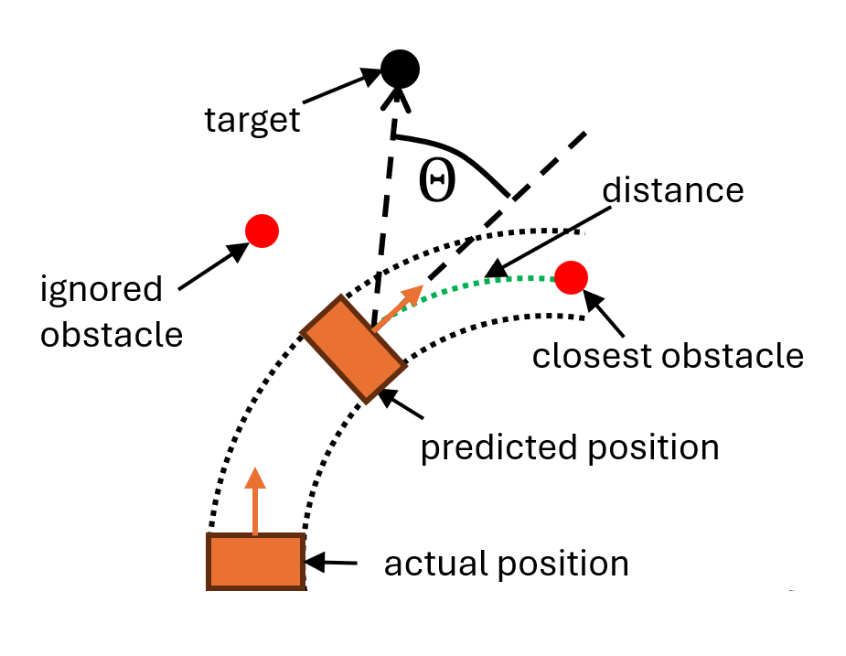
DWA performs reactive collision avoidance. When computing the next moving command, DWA considers only a short time interval, within which the robot's velocities [math]\displaystyle{ (v, \omega) }[/math] are considered to be constants. The algorithm will evaluate the results of all possible velocities and select the optimal one. Instead of using the simplified version introduced in lectures, we use the original version of this algorithm proposed by D. Fox, etc. The main difference is that the original algorithm uses a more refined geometric model when calculating the distance between the obstacle and the predicted trajectory, taking both the trajectory and the robot size into account. As shown in figure on the right, the obstacles that are not on the trajectory will be ignored. And by including a safety margin, we can control the minimum distance between obstacles and Hero.

The set of all possible velocities [math]\displaystyle{ V_r }[/math] is called the search space. It is the intersection of three sets: [math]\displaystyle{ V_r = V_s\cap V_a\cap V_d }[/math], where [math]\displaystyle{ V_s }[/math] is the set of velocities that are limited by robot's dynamics, [math]\displaystyle{ V_a }[/math] is the set of velocities with which the robot can stop before reaching the closest obstacle and [math]\displaystyle{ V_d }[/math] is the set of velocities constrained by current velocities and acceleration.

These three sets are defined as:

[math]\displaystyle{ \begin{align} \begin{matrix} V_s =&\left\{v,\omega |v\in[v_{min},v_{max}]\wedge \omega\in[\omega_{min},\omega_{max}] \right\}\\ V_a =&\left \{v,\omega |v\le \sqrt{2d(v,\omega )\dot{v}_b } \wedge \omega \le \sqrt{2d(v,\omega )\dot{\omega }_b} \right \}\\ V_d =&\left \{v,\omega |v\in [v_{a}-\dot{v}\Delta t,v_{a}+\dot{v}\Delta t] \wedge \omega \in [\omega_{a}-\dot{\omega}\Delta t,\omega_{a}+\dot{\omega}\Delta t] \right \} \end{matrix} \end{align} }[/math]

where [math]\displaystyle{ \dot{v}_b }[/math] and [math]\displaystyle{ \dot{\omega }_b }[/math] are maximum deceleration values and [math]\displaystyle{ d(v,\omega) }[/math] is the distance to the closest object; [math]\displaystyle{ v_a }[/math] and [math]\displaystyle{ \omega_a }[/math] are actual velocities and [math]\displaystyle{ \dot{v} }[/math] and [math]\displaystyle{ \dot{\omega} }[/math] are maximum acceleration values.

[math]\displaystyle{ V_s }[/math] and [math]\displaystyle{ V_d }[/math] ensure that the selected reference velocities is consistent with the physical limitations of the robot. And [math]\displaystyle{ V_a }[/math] ensures that the robot does not collide, because the distance item of velocities that lead to collision will be zero, making these velocities unavailable.

Implementation in C++

Pseudo code of DWA

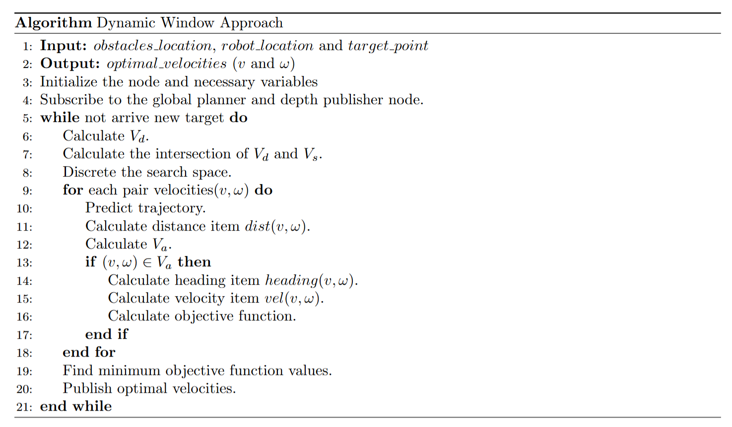
As shown in the figure on the right, the DWA is basically a discrete search to maximize the reward function. Considering the large number of parameters of DWA, we implement DWA as a class in C++ and make those parameters as class-scope private constants. There are two advantages to such an implementation.

Firstly, with the limitation of class scope and constant private variables, these parameters will not be accessible to other code, which guarantees these parameters will not be modified by other code and helps to improve code clarity.

Secondly, packaging all the parameters of DWA in a single class helps to improve the portability of the code. One can easily use this code by including a head file. And if we want to change these parameters only, we can simply re-compiler this part solely and then link it with others, instead of re-building the whole project. The reason we didn't use a file (such as JSON or XML) to configure these parameters is that we want the compiler to perform compile-time constants optimization, as these parameters should be known constant in the final challenge.

Parameter Tuning

Simulation Results

Test on Hero

Interaction

(Lu)

Final Challenge Results

Results Analysis

（Hao）

Future Improvement

（Nan）