Embedded Motion Control 2014 Group 3
Group Members
| Name: | Student id: |
| Jan Romme | 0755197 |
| Freek Ramp | 0663262 |
| Kushagra | 0873174 |
| Roel Smallegoor | 0753385 |
| Janno Lunenburg - Tutor | - |
Software architecture and used approach
LaserProcessing
LaserData from Pico
The data from the laser on pico is in lasercloud format. This means that the data is represented in an array of distances. The starting angle and angle increment are known. This means we have the distances from laser to objects for a range of angles.
LaserCloud to Pointcloud
Because we are going to fit lines through the walls, it would be easier to have the data in Carthesian Coordinates. In this node the laserData is transformed into a PointCloud, which is published on the topic. It is also possible to filter the data in this node when needed. For now all data is transformed into the PointCloud.
Arrow detection
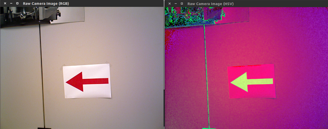
The following steps describe the algorithm to find the arrow and determine the direction:
1. Read rgb image from "/pico/asusxtion/rgb/image_color" topic.
2. Convert rgb image to hsv color space.
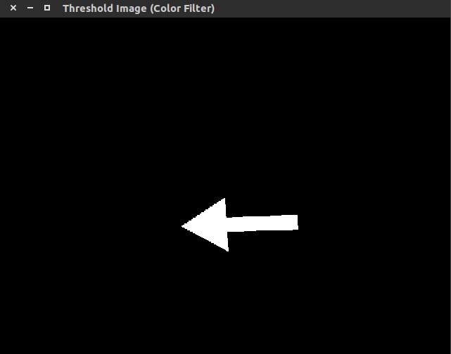
3. Filter out the red color using cv::inRange
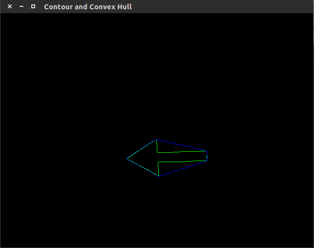
4. Find contours and convex hulls and filter it
The filter removes all contours where the following relationship does not hold: [math]\displaystyle{ 0.5 \lt \frac{Contour \ area}{Convex \ hull \ area} \lt 0.65 }[/math]. This removes some of the unwanted contours. The contour and convex hull of the arrow:
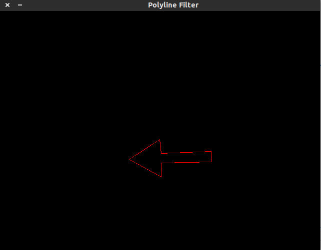
5. Use cv::approxPolyDP over the contours
The function cv::approxPolyDP is used to fit polylines over the resulting contours. The arrow should have approximately 7 lines per polyline. The polylines fitted over the contours with [math]\displaystyle{ 5 \ \lt \ number \ of \ lines \ in \ polyline \ \lt \ 10 }[/math] is the arrow candidate.
6. Determine if arrow is pointing left or right
First the midpoint of the arrow is found using [math]\displaystyle{ x_{mid} = \frac{x_{min}+x_{max}}{2} }[/math]. When the midpoint is known the program iterates over all points of the arrow contour. Two counters are made which count the number of points left and right of [math]\displaystyle{ x_{mid} }[/math]. If the left counter is greater than the right counter the arrow is pointing to the left, otherwise the arrow is pointing to the right.
7. Making the detection more robust As last an effort is made to make the arrow detection more robust, for example when at one frame the arrow is not detected the program still knows there is an arrow. This is done by taking the last 5 iterations, check if in all these iterations the arrow is detected then publish the direction of the arrow onto the topic "/arrow". If in the last 5 iterations no arrow is seen the arrow is not visible anymore thus publish that there is no arrow onto the topic "/arrow".
PFM
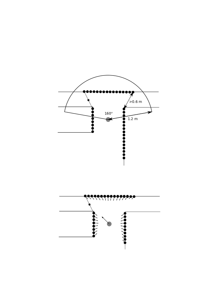
For robustness, it was decided to use a Potential Field Method (PFM). This means that a low potential is assigned to the setpoint, while the detected obstacles have a high potential. A loop over all points [math]\displaystyle{ i }[/math] in the pointcloud calculates their repulsive force in Carthesian components([math]\displaystyle{ Fx }[/math] and [math]\displaystyle{ Fy }[/math]), and the force is normalized using the distance [math]\displaystyle{ d }[/math] to the point.
[math]\displaystyle{ d_i=\sqrt{x_i^2+y_i^2} }[/math]
[math]\displaystyle{ Fx_i=-0.7*\frac{1}{d_i^5}*x_i }[/math]
[math]\displaystyle{ Fy_i=-0.7*\frac{1}{d_i^5}*y_i }[/math]
Every point in front of Pico that has a distance smaller than 1.2 meters from Pico will trigger a check to see if the next point of the pointcloud is more than 0.6 meters away from the previous point. If so, the jump in distance is assumed to relate to a door, and the setpoint is placed in the middle between the two points. The some of all the repulsive forces is added to the attracting force of the chosen setpoint and normalized.
Organization
Time survey
Link: time survey group 3
Planning
Week 1 (28/4 - 4/5)
Finish the tutorials
Week 2 (5/5 - 11/5)
Be able to detect walls and convert them to start and end points
Week 3 (12/5 - 18/5)
Finish strategy to be able to successfully finish the competition
Older Software
Overview of first strategy
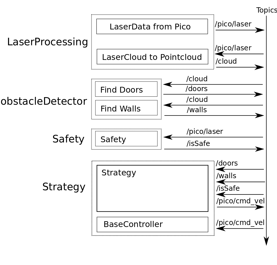
In the overview the different packages (dotted boxes) and nodes (solid boxes) are displayed. The topics are displayed at the sides of the nodes.
Initial (boolean) safety
The safety node is created for testing. When something goes wrong and Pico is about to hit the wall the safety node will publish a Bool to tell the strategy it is not safe anymore. When the code is working well safety shouldn't be needed anymore.
Obstacle Detection
Finding Walls from PointCloud data
The node findWalls reads topic "/cloud" which contains laserdata in x-y coordinates relative to the robot. The node findWalls returns a list containing(xstart,ystart) and (xend, yend) of each found wall (relative to the robot). The following algorithm is made:
- Create a cv::Mat object and draw cv::circle on the cv::Mat structure corresponding to the x and y coordinates of the laserspots.
- Apply Probabilistic Hough Line Transform cv::HoughLinesP
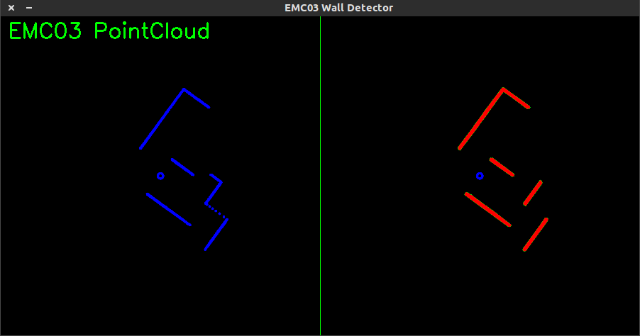
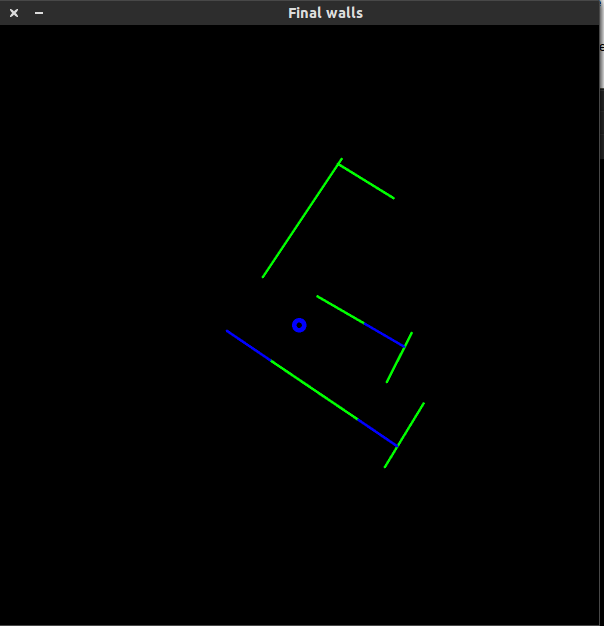
In the picture shown below one can see the laserspots at the left side of the picture. At the right side the lines of the cv::HoughLinesP are shown.
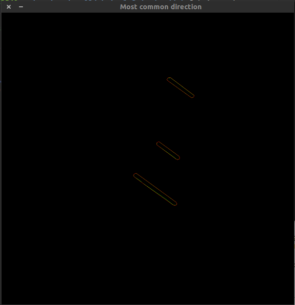
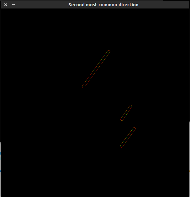
The cv::HoughLinesP algorithm gives multiple lines per wall. In the end we want 1 line per wall. To solve this first the all the lines are sorted into lists by their angle they make, for example if a line makes angle of [math]\displaystyle{ 27^\circ }[/math] it is stored in a list where all lines lie between [math]\displaystyle{ 20^\circ }[/math] and [math]\displaystyle{ 30^\circ }[/math]. Once all lines have been sorted the two most common directions are plotted which is shown in the following pictures:
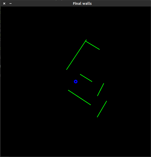
Finally to extract 1 line per wall the outer points of the contour are taken to get 1 line per wall. The result is shown in the following figure:
Finding Doors from found Walls
Now that the walls are given as lines doors are fitted between the walls. The result is shown in the following figure:
Why this method doesn't work in real life
The method described in how to find walls and doors did not work properly in real life. We experienced some serious robustness problems due to the fact that in some of the iterations complete walls and/or doors were not detected, thus the robot couldn't steer in a proper fashion to the target. Secondly this method required some serious computation power which is not preferable (one cpu core ran at 80% cpu when the refresh rate of the algorithm was only 5 Hz).
Overview of second strategy
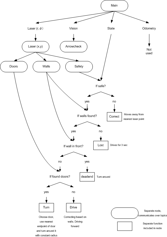
See diagram, circles represent separate nodes that communicate using topics. Blocks represent functions, which will be written in separate c++ files and included in the "main" c++ file. This way, no one will interfere in code of someone else.
Notes (TODO)
Week3
Combine detection and strategy part
+ Determine waypoint (turnpoint)
- Find door (using end of line)
+ Turn
+ Drive out of maze
Week 4 (week after corridor challenge)
Because of the Elevator project Freek is not responsible for anything this week.
Jan and Roel will write (optimize) the wall finding algorithm and use it also for the doors. Kushagra will write the safety node.
