Mobile Robot Control 2020 Group 2
Mobile Robot Control 2020 Group 2
Group members
Marzhan Baubekova - 1426311
Spyros Chatzizacharias - 1467751
Arjun Menaria - 1419684
Joey Verdonschot - 0893516
Bjorn Walk - 0964797
Bart Wingelaar - 0948655
Introduction
This is the wiki page of the Group 2 of the Mobile Robot Control course of 2020. The page contains all the information regarding the assignments accomplished within the course including the plan, procedure, algorithms, implementation and results. During the course we have been introduced to a software design and how to apply this in the context of autonomous robots. There are two assignmnets, which are done and reported here, namely Escape Room challenge and Hospital challenge. Unfortunately, due to the circumstances caused by the Corona virus, we were unable to apply the software on real robot, however, the simulation was adapted by the tutors to the real-life environment as much as possible.
The first task was to develop a design document which is the first step in the software development and requires the understanding of the problem, evaluation of the robot specifications and its environment, and software components. Next, from the document we proceeded to the implementation of the software for the Escape Room Challenge. After succesful accomplishment of the first challenge, we moved to the design of the software for the Hospital Challenge. Finally, the results are evaluated and conclusions are drawn.
Design Document
The design document for the escape room challenge can be found here:
File:Mobile Robot Control Design Document Group2.pdf
Escape Room Challenge
The goal of the escape room challenge is to find the exit of a room autonomously and 'escape' the room through the exit corridor without bumping into the walls. In this challenge the robot is placed in a rectangular room, which dimensions as well as the initial position of the robot in the room are not known. In order for the robot to succeed in this challenge, a design document was created first, which includes the requirments & specifications, components, functions and interfaces.
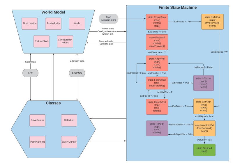
As stated in the design document, the software of the robot is developed based on a finite state machine. The finite state machine will start in a predefined initial state and will go to next states if certain conditions are met. The finite state machine will follow the states until the final state is 'finished'. While going through these states, the robot communicates with the world model. The main functions of the world model are to store important information and to share it between all classes.The information stored in the world model is for example the direction of the exit when identified or the distance to a wall. The other classes determine the actual actions of the robot. The SafetyMonitor will retrieve for example the distance to a wall and determine if the distance is larger than a certain threshold. If the wall is too close, the SafetyMonitor will tell the robot to move away from the wall to get some clearance. The detection class retrieves the laser data and determines the distances to walls or finds the exit. These parameters are then stored in the world model. Drive control determines the movement of the robot. Path planning is not used in the escape room but will be used for the hospital challenge.
At the start of the escape room challenge the robot will start to scan the room. This scan is then analyzed to determine if the exit can be seen. If the exit is detected, the robot will move in the direction of that exit until it gets close to the exit. If the exit can not be seen, the robot will rotate approximately 180 degrees to do a second scan. If the exit is detected now, the robot will move as it would if during the first scan a exit was detected. If in the second scan the exit can still not be identified, the robot will move to the closest wall found in both scans and start to follow this wall using a wall following algorithm.
When the exit is found from one of the initial scans, the robot will rotate to face the correct direction towards the exit. It will then start to move forward towards the exit. When it gets close to a wall the robot assumes it is near the exit and starts the exit alignment procedure. This exit alignment procedure makes sure that the robot will enter the hallway approximately in the middle to stay clear of the walls. When the alignment is done the robot will start the exit entering procedure.
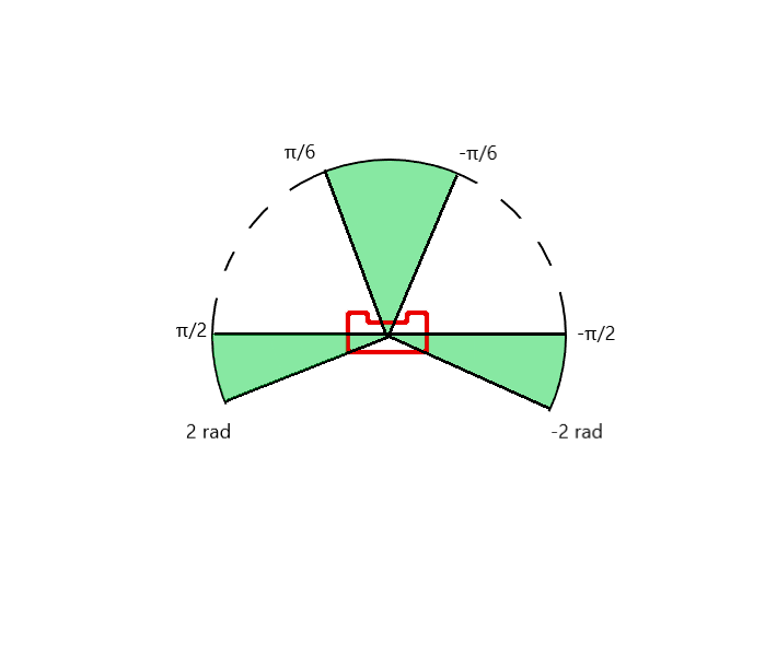
The wall following algorithm makes the robot move in a clockwise direction. When it gets close to a corner it will rotate approximately 90 degrees and use the wall to the left to correct and align to an almost perfect 90 degrees. When it suddenly sees a jump in the distance of the wall to the left, it detects this as the exit. The robot scans a larger part of the wall while driving to identify this gap. This also means that if it is only a small slit in the wall, it will not detect this slit as a exit. When the robot has then moved forward so that it is standing in front of the gap, it will rotate to face the gap. It will then align so that it is standing approximately in the middle of the gap and start the exit entering procedure.
The exit entering procedure makes sure the robot slowly drives forward until it is somewhat into the hallway. While it is doing this, it is scanning for walls to the left and right of the robot to make sure it will not hit any walls. If the robot gets to far out of the middle line of the hallway, it will reposition itself towards the middle. While in the hallway the procedure is quite similar with respect to aligning to the middle line of the hallway. In the hallway the robot will also align to be parallel to the left wall of the hallway. This is done to make sure the robot can not get to close to this wall. Combined with staying in the middle line of the hallway, this ensures that the robot will not hit any of the walls in the hallway.
While in the hallway the robot will also scan ahead slightly to the left and right. This is done to determine when the robot has crossed the finish line. When the robot no longer sees walls in the front left and right direction, it will assume that it has crossed the finish line.
A flow chart of finite state machine is shown below:
In the live Escape Room challenge the robot did not finish. In the first attempt this was due to the fact that the robot started close t0 the wall. This scenario was unfortunately not tested. The robot starts by scanning the room and trying to find the exit. When an exit is found the robot moves towards it. However, the criteria for the robot to determine that it was close to the exit was if a wall is nearby. This criteria works if the robot starts cleared of the walls and can drive straight to the exit. Since the robot started close to a wall in the challenge, it immediately thought it was at the exit and tried to allign with the hallway. This obviously did not work since there was no hallway.
The second attempt was a simple wall following algorithm. However, again a specific case was not tested making the robot still not finish the challenge. In this case it was the situation where the exit was very close to a corner. When the robot gets to a corner it is supposed to rotate approximately 90 degrees, and then use the wall to the left to align with the wall. Now that the exit was close to the corner, it could not detect the wall to align with, and the software got stuck in a loop.
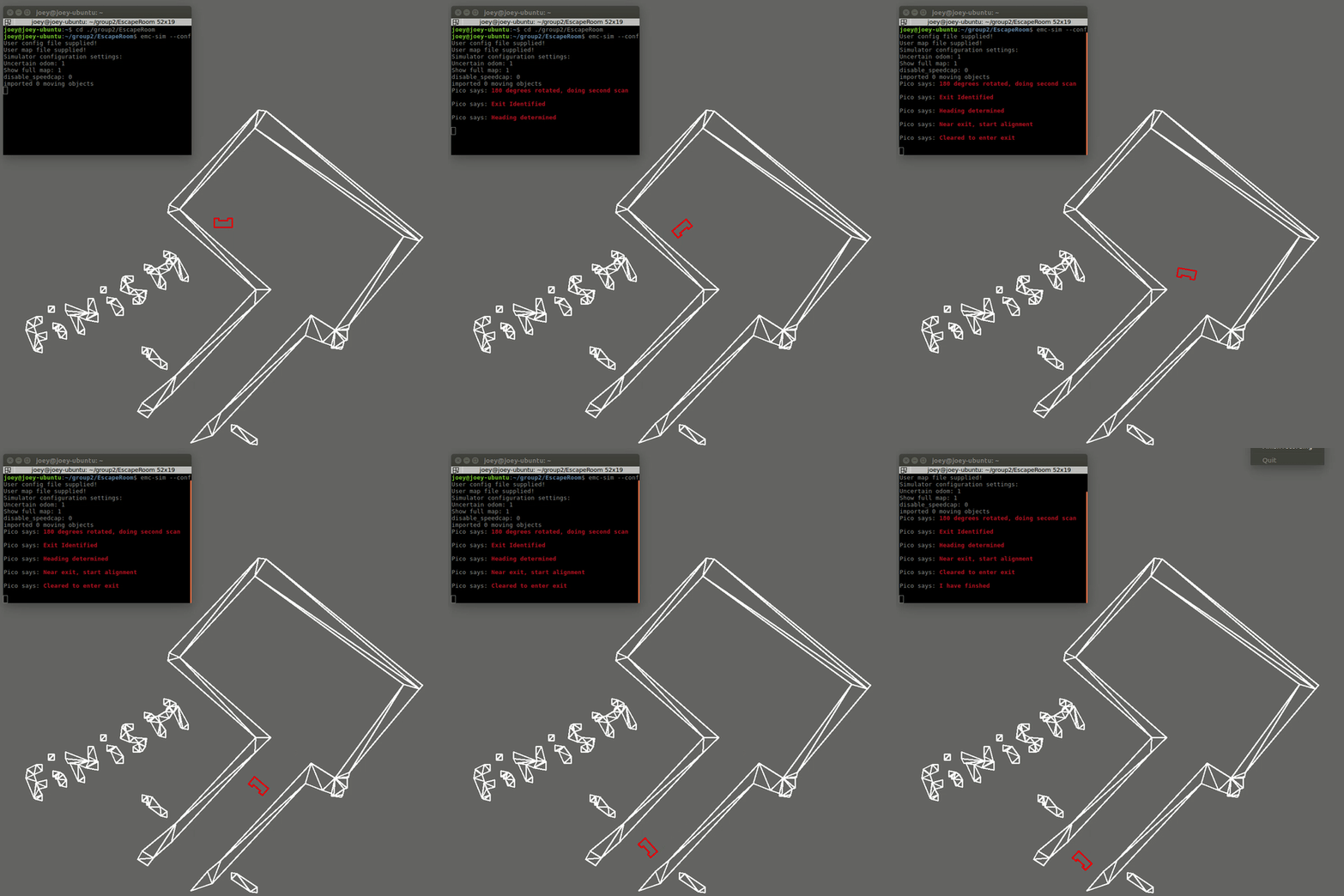
The first code was fixed by changing the criteria for when the robot assumes it is close to the exit. Now the distance to the exit is measured at the 20Hz sampling rate. This distance was already calculated in the original code, however it was not stored and used. Now that it is used, the robot will only start the alignment procedure for the hallway when this distance is below a threshold. The robot will also move away from the wall slightly after the scanning to ensure safety margins. This was already in the code, but was not executed since the robot never started moving but immediately thought it was at the exit. The result is now that the robot escapes the room in 19 seconds and stops right after crossing the finish line and speaks "I have finished". The result is shown below:
Hospital Challenge
Path Planning
The path planning is an essential component in this challenge. This component links the current position and orientation in the global map to the destination: cabinets. On its path, this componenth has to deal with static and dynamic objects and closed doors.
Algorithm selection
For the selection of the algorithm used for path planning, several algorithms have been considered: A*, Dijkstra, Rapidly-exploring random tree, wall following, wave propagation and Potential field algorithm. Each of these algorithms has its pros and cons, so they have been evaluated at several criteria that were relevant for the hospital challenge. This trade-off is presented in the table below.
The first 2 criteria are closely related. The speed of the algorithm is important, as hardware performance is limited. The ‘speed’ column contains some notes of the method of the algorithm. The compute index quantifies this criteria to compare it, as the speed criteria is relatively important. The compute index is based around A* which is given an index number of 100. The walls and Dijkstra compute indices are an educated guess. The others are based on the amount of nodes used in a study. The others are based on the amount of nodes used in a study. In the robustness criteria the algorithms are evaluated whether or not it can find a path at all. Path smoothness is important, as too many sharp turns can introduce a drifting error in the orientation in case of odometry feedback. It also influences the speed of the PICO robot, as it may need to stop to rotate. The implementation criteria evaluates the convenience of implementation. All team members have experience with some algorithms already, which accelerates implementation and unfamiliar algorithms can introduce implementation challenges due to the novelty factor. The implementation can also be hard, regardless of previous knowledge in case the algorithm needs to account for a large number of situations/cases.
Based on these criteria, the A* algorithm is selected. It is not the fastest, yet relatively fast. Its path is relatively smooth. Experience with this algitithm makes the implemnation less complicated
| Algorithm | Compute index | Speed | Robustness | Path smoothness | Implementation | General notes |
|---|---|---|---|---|---|---|
| A* | 100 | +fast, +direct (it does not explore all the space) | +finds descent short path if it exists | -+relatively smooth, depends on grid and allowed movements | + known method | path update when obstacle detected |
| Rapidly-exploring random tree | 100 | -expands in all the space | +finds shortest path if it exists | +relatively smooth | -unknown method | good with dynamic objects |
| Potential field algorithm | 40 | -fails in case of local minimum | +relatively smooth | -unknown method | ||
| Dijkstra | 100 or higher | -slower than A*, -expands in all the space | +finds shortest path if it exists | -+ relatively smooth, depends on grid and allowed movements | + known method | path update when obstacle detected |
| Wall following | 100000 | -slow | - prone to fail in case of blocking objects | -smooth, but discontinuities exist | - difficult with many cases to account for | copy parts from escape room challenge |
| Wave propagation | 100 or higher | expands in all the space | +finds shortest path if it exists | + relatively smooth | +similar to A* | path update when obstacle detected |
Implementation
The A* algorithm is based on an existing algorithm which has been modified. An import factor in the A* algorithm is the heuristic and a well selected heuristic ensures performance and efficiency. The default heuristic in the used algorithm is the Euclidean norm with respect to the destination. With 8 movements possible from each node(diagonal,left,right,front back movement), this is not the fasted, according to a article on heuristics. A diagonal heuristic is more suitable for these allowed movements.
The algorithm uses a binary regular grid map. In parallel a regular coordinate grid map has been developed to represent the global map of the hospital. The initial position and orientation is unknown and follows from the initial localization. It may be that it does start on a node and/or is not aligned with the path that the A* algorithm gives. To account for this the path is ‘extended’ in case it is not within 25 mm radius of a node. As the map has a regular sized grid, it evaluated multiple close nodes , in case it does not start on a node. Then it selects the path of the closest node which give the shortest path to the destination. Subsequently, if needed, extra rotation is applied to align with the path.
The grid map is illustrated in the figure below. A safety margin from the walls and cabinets of 30cm is applied in the positioning of the nodes. One can observe that there are many nodes, many of which will likely never be used. They are still there to account for any objects that might arise in the hospital challenge and require a detour using these nodes to avoid collision with objects on its path.

User interaction
The user interaction is different than mentioned in the challenge requirements to benefit the user experience. The user is asked for the input with an example and feedback is given. This benefits the user experience. The user interaction interface is illustrated in the figure below.

Motion Control
Localization
For successful navigation it is important that the robot is aware of its current location. After considering known algorithms such as Markov localization, Kalman filter and particle filters, it has been chosen to implement the line segment based localization. (Why?? restricted in time, experience, identification of landmarks is problematic and etc.)
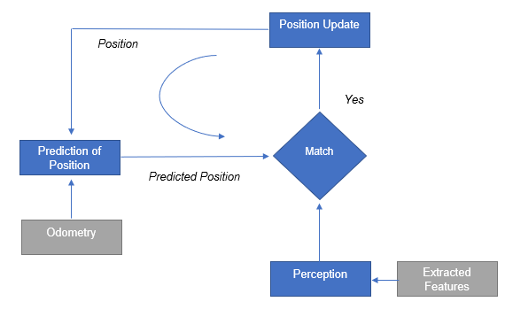
Before the localization can work, an initial pose needs to be determined. This is done using known landmarks. In this case the door of the room where the robot starts is used. The laser data is analyzed to find the door in the same way it is done in the Escape room challenge. When the door is found, the robot will rotate to face the exact middle point of the door. This is done to be able to also determine an angle. When the robot faces this middle point, the sides of the door are found in the laser data. Using the range and the angle for these points, the x-y position can be determined using trigonometry. When the initial position is known, combined with knowing the location of the middle point of the door the robot is facing, the initial angle can be determined completing the initial estimation of the pose. The algorithm is made robust such that it can not falsely identify other objects in the room or small gaps in the walls as the door. The accuracy of the initial pose is dependent on the accuracy of the LRF. However, this initial localization is only used to get a first estimation of the pose, and the actual localization function will use this and correct it based on all the data it retrieves.
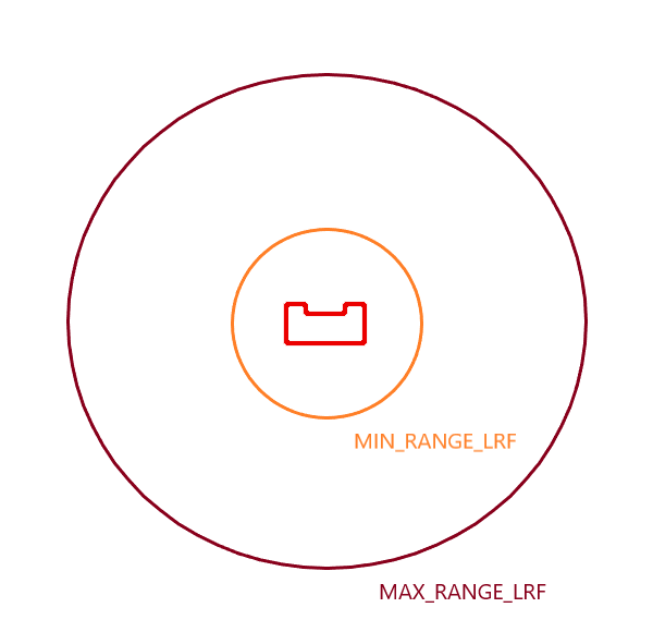
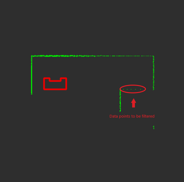
| Split and Merge Algorithm: |
|---|
| Initialize segments set S. |
| 1. Filter LRF outliers by setting thresholds MAX_RANGE_LRF and MIN_RANGE_LRF. |
| 2. Convert LRF data to cartesian coordinates. |
| 3. Calculate the distance between two cartesian points and check if it is within threshold DUMP_DIST. |
| 4. Check for a jump in LRF ranges of the filtered data set and if the jump is bigger than threshold CLUSTER_MARGIN-> make segmentation |
| Split |
| 1. Fit a line to begin and endpoint in current set S. |
| 2. Find the most distant point to the line using heron's formula. |
| 3. If distance > threshold LSE_MARGIN, then split and repeat with left and right point sets. |
| Merge |
| 1. If two consecutive segments are close/collinear enough, obtain the common line and find the most distant point. |
| 2. If distance <= threshold, merge both segments. |
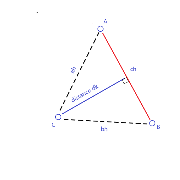

In our case the base b is ch and h is a distance-to-be-found dk. Area A is calculated by Heron's formula since all three distances ah, bh and ch can be found. To calculate area, define first

then

Finally, the distance can be calculated:

The initial choice for localization method was the Extended Kalman Filter (EKF) because its implementation is considered easier than other methods, such as the Particle Filter and its probabilistic approach can lead to more accurate estimation than other methods, such as line segment localization. Unfortunately, due to limited amount of time the implementation of EKF did not provide robust results for localization and therefore it was not implemented in the main code for the hospital challenge. However, the method was applied and tested on a simplified example, where the real position of the robot was estimated during its movement from one known point in the map to another point. The basic steps of the EKF algorithm as implemented for the hospital challenge are described in the following paragraphs. A code sample of the simplified example is attached at the end of this wiki page.
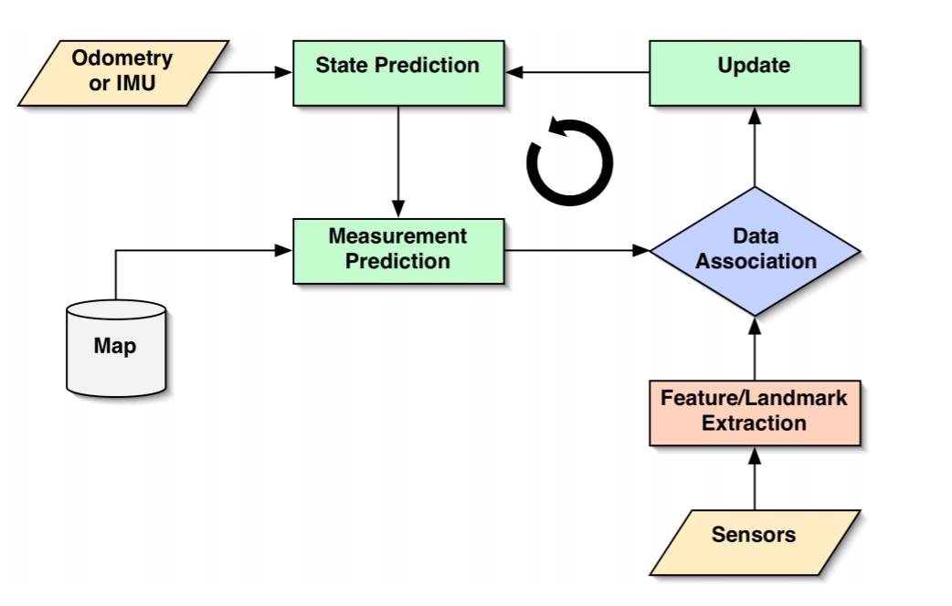
Stage prediction: For the implementation of the EKF a prior knowledge of the initial position of the robot is required (x,y and theta with respect to the global frame of the hospital map). This is provided by the initial localization module, which was described in a previous section (IS IT ???). The first step of the algorithm (Stage Prediction) takes into account the given initial position of the robot and it calculates a predicted position by adding the odometry data (Odometry) given by the encoders (assuming that the odometry data are accurate, without any errors). The equations for state prediction and state covariance are:
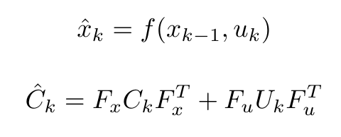
where u_k is the displacement vector and U_k the variance matrix for the inputs, given as follows:
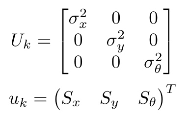
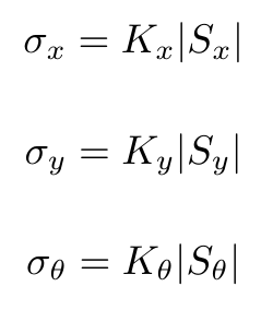
Measurement prediction: At the measurement prediction stage the position of the the known corners with respect to the global map frame (map) are expressed with respect to the predicted position of the robot. This transformation of every known corner (i) of the map is demonstrated as the following function:

Landmark extraction:
At landmark extraction the data from the laser sensors are used in the split and merge algorithm, as described in a previous section, in order to calculate the position of the corners inside the laser range with respect to the robot frame (Cartesian coordinates). The position vector of each observed corner (j) and the observation uncertainty matrix are described as follows:

Data association: At the data association stage the observed corners from the Landmark Extraction stage are matched with the known corners from the map. The difference of the position of observed and known corners with respect to the robot frame are calculated and saved in the innovation vector v_k. For every possible match up, if the difference is smaller than a specified threshold then the observed corner is identified. If the observed corner is not matched up with any of the known corners (i.e. in the case of an unknown static or dynamic object) then the corner is ignored and the algorithm continues with testing the next possible match up. A different approach of this algorithm uses the information of the unmatched corners to identify and locate unknown objects. For the purposes of the hospital challenge this information is ignored, since the object detection is dealt with a different method. The innovation vector and the innovation covariance matrix are described as follows:
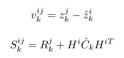
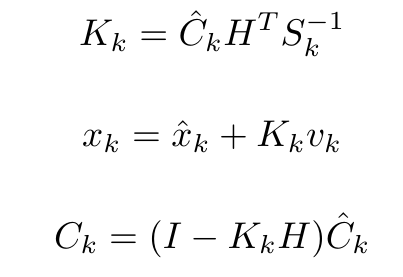
Update: At this stage of the EKF algorithm the position of the robot, the state covariance and the vector with the Kalman gains are updated. The composite innovation Vk, the composite innovation covariance Sk and the composite of the measurement prediction function H are calculated from vk_ij, Sk_ij and Hi respectively. The update equations are:
Visualization
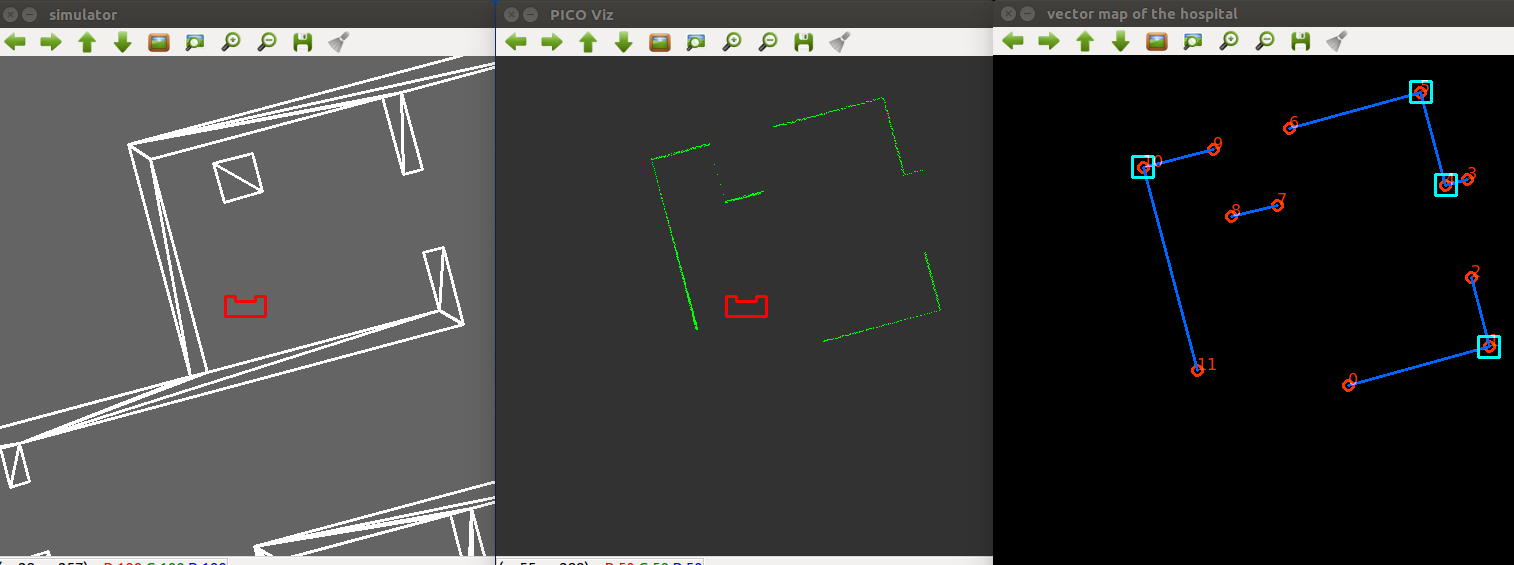
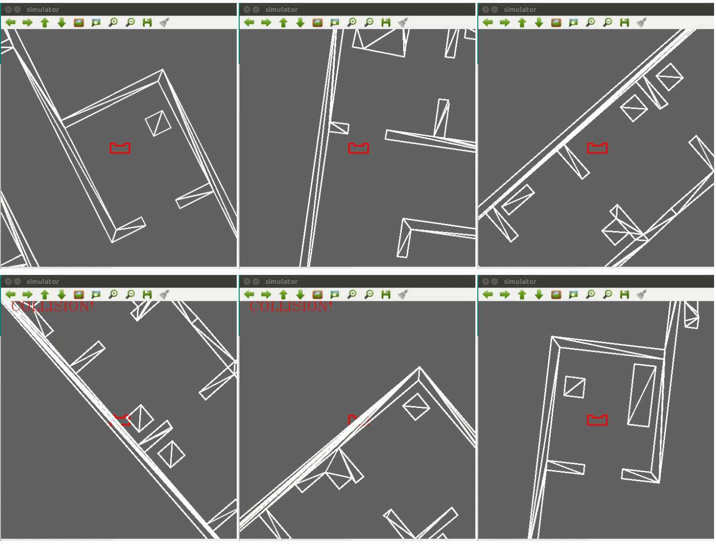
In order to debug the code in a more efficient way, the map and important functions of the code are visualized with a visualization class using the openCV library. In the beginning of the code a white canvas is created in a separate window where the map will be visualized from the provided JSON file. Then this code is extended to visualize the important functions each time these functions are called, the considered functions in this case are the pathplanning and the line & corner extraction of the robot's laserdata. Furthermore, a second window is created in which the laserdata in front of the cabinet, is visualized, as it should be saved as a different image for each cabinet.
The visualization is made using basic functions of the openCV library such as imshow() and imwrite(). Furthermore different structures are made for each specific object such as the cabininets, walls, corners, etc, in order to visualize the correct associated data.
Results and Discussion
Logs
| Meeting # | Date and Location | Agenda | Meeting notes |
|---|---|---|---|
| 1 |
Date: 28-04-20 Time: 10:00 Platform: MS Teams |
|
|
| 2 |
Date: 01-05-20 Time: 14:00 Platform: MS Teams |
|
|
| 3 |
Date: 05-05-20 Time: 10:00 Platform: MS Teams |
|
Work division
|
| 4 |
Date: 11-05-20 Time: 11:00 Platform: MS Teams |
|
Work division
|
| 5 |
Date: 18-05-20 Time: 11:00 Platform: MS Teams |
|
Work division
|
| 6 |
Date: 22-05-20 Time: 14:00 Platform: MS Teams |
|
Work division is the same
|
| 7 |
Date: 26-05-20 Time: 11:30 Platform: MS Teams |
|
Work division is the same
|
| 8 | 5 | 10 | 15 |