Mobile Robot Control 2020 Group 7
Group Members
| Name | Student Number | |
|---|---|---|
| 1 | Mick Decates | 0957870 |
| 2 | Steven Eisinger | 1449273 |
| 3 | Gerben Erens | 0997906 |
| 4 | Roohi Jain | 1475061 |
| 5 | Mengqi Wang | 1449435 |
| 6 | Goos Wetzer | 0902160 |
Introduction
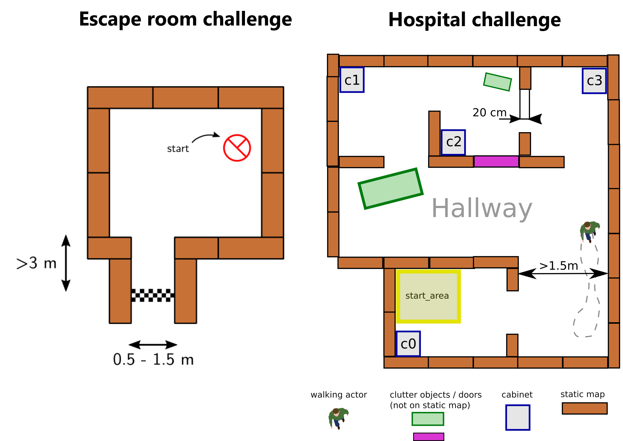
Welcome to the wiki of group 7 of the 2020 Mobile Robot Control Control course. During this course the group designed and implemented their own software which allows a PICO robot to complete two different challenges autonomously. The first challenge is the "Escape room challenge" where the PICO robot must drive out of the room from a given initial position inside the room. In the second challenge called the "Hospital challenge" the goal is to visit an unknown number of cabinets in a specific order, placed in different rooms. For both challenges the group designed one generic software structure that is capable of completing both challenges without changing the complete structure of the program. The example maps of both challenges are shown in Figure 1 to give a general idea about the challenges. The full details of both challenges are given on the general wiki page of the 2020 Mobile Robot Control course (link).
Escape room challenge
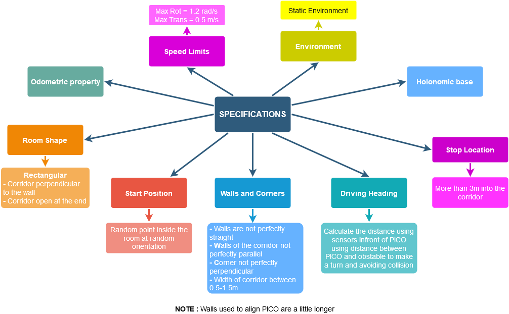
The main goal of the challenge was to exit the room as fast as possible, given an arbitrary initial position and orientation of PICO. The robot will encounter various constraints such as the length of the finish line from the door, width of the hall way, time constraints and accuracy. The PICO robot was first placed in a rectangular room with unknown dimensions and one door/opening towards the corridor. The corridor was perpendicular to the room with an opening on its far end as well. The initial position and orientation of the PICO robot was completely arbitrary. PICO was supposed to cross the finish line placed at a distance greater than or equal to 3 metres from the door of the corridor. The walls of the room were also not straight which posed a challenge during the mapping of the room from the laser data. The challenge is discussed in much detail about the algorithms used, implementation, program flow and results of the challenge in the following sections.
Hospital challenge
The main goal of this challenge was to visit the cabinets in a particular order given by the user as fast as possible. The global map consisting of rooms and cabinets and the starting room of PICO were mentioned beforehand. The hospital challenge contained multiple rooms with doors which can be open or closed. It tested the ability of PICO to avoid static/dynamic objects and plan an optimal path dynamically. The static objects included clutter objects/doors and the dynamic objects included human beings moving in the room while PICO was performing its task which were not specified on the given global map. Lastly, PICO was asked to visit the list of cabinets to visit in a specified order given by the user before the start of the challenge. The challenge is discussed in much detail in the following sections. The algorithms used are explained, how they are implemented is shown, the program flow is discussed, and the results of the challenge are told.
Hardware Components
Sensors - Laser Range Finder
The laser range finder measures the distance from the robot to the closest obstacle for a range of angles around the direction the robot is facing. The sensor data is stored in a structure called LaserData, which is described in table 3.1. There are 1000 measurements in total.
| Property | Description |
|---|---|
| range_max | The maximum range that can be measured is 10 meters |
| range_min | The minimum range that can be measured is 0.01 meters |
| angle_max | 2 radians from the direction straight ahead |
| angle_min | -2 radians from the direction straight ahead |
| angle_increment | Each angle is 0.004004 radians away from the next one |
| timestamp | Timestamp of the measurement in UNIX |
Sensors - Odometry
The odometry data measures the distance the robot has traveled in all 3 degrees of freedom in the horizontal plane.This data is obtained through encoders on the wheels of the holonomic base, which are stored in a structure called OdometryData, described in table 3.2. Small errors could accumulate over time due to measurement errors and wheel slip. To combat this, the positional data of the robot will be updated using the difference between the current and previous odometry measurement. This data is then corrected with the use of the world model and the data obtained from the laser range finder.
| Property | Description |
|---|---|
| x | distance travelled in horizonal direction since start of measurement |
| y | distance travelled in vertical direction since start of measurement |
| a | angle rotation since start of measurement |
| timestamp | Timestamp of the measurement in UNIX |
Actuators
The robot is built on a holonomic base, which means that it has three degrees of freedom in its horizontal plane: twotranslational, and one rotational. The robot is able to move in these ways using its omni-directional wheels, which are placed in a triangular formation on the base. Besides being able to provide a force in the driving direction,unlike normal wheels, the omni-directional wheels also do not constrain movement in the direction orthogonal tothe driving direction. Because of this, the robot is able to move with a given max velocity in all possible directions of the horizontal plane.
ESCAPE ROOM CHALLENGE
Requirements & Specifications
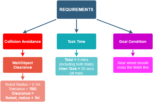
The requirements and specifications for the challenge are shown in figure. The primary requirement is safety that we need to fulfill by avoiding collision. All other requirements shall be treated equally.
Functions
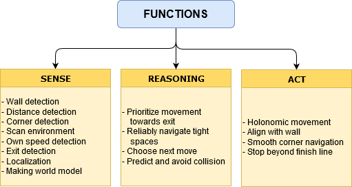
Once the robot is deployed in the room, it should sense around the room and try to find the exit corridor. If it cannot find the corridor, it should move around the room in an attempt to find it. Once the corridor is found it should position itself in front of the corridor and proceed through it until crossing the finish line.The functions that the robot needs to perform these tasks are described in Figure 2.1. These functions are divided into three main components: Sense, which allows the robot to perceive and quantify its world; Reasoning, where the robot makes a decision based on its perception; and Act, which determines what action the robot performs based on its reasoning information.
Software Infrastructure
The software will be divided into components, which are connected through certain interfaces. Major components are seen in Figure 5, and their interfaces are specified with the arrows. Perception is the component where the PICO uses sensor data from LaserData and OdometryData to get an idea of it’s current location. This data is interfaced with the World Model, which stores map and localization data, including the exit location once found. The Planning component takes care of decision making and control planning, including path finding and obstacle avoidance. The actuation component will actuate the holonomic base in order to carry out the movement plan.

Implementation

The overall software behavior is divided in five clearly distinguished phases. During each phase all actions lead to one specific goal and when that goal is reached, a transition is made towards the next phase. The overall program logic can be seen in Figure 6.
Initialization
This is the first phase of the robot as soon as the software is run. All the inputs and outputs of the robot are initialized and checked, during this phase. Moreover, all the required variables in the software are set to their correct values. At the end of the initialization phase the software is set and ready to perform the desired tasks. The first task of the robot is to find the wall and align with it.
Find wall and align with wall
When the robot is initialized in its environment, the first thing that the robot will do is find the wall that is the closest to him. The way that this has been implemented is by first scanning all the distances over a certain angle using the LRF. During this scan, the robot will store the value that has the shortest distance, along with the corresponding angle. These two values are returned, and the robot will check whether this value is in front of him or not. If the shortest distance is not in front of him, then the robot will rotate over the shortest angle, until it faces the shortest distance between him and the wall. Once the robot is facing the shortest distance, it will start moving towards it until the shortest distance value passes a given minimum value. This is so that the robot does not collide with the object in front of him. During this procedure, the robot is constantly updating its laser data in order to obtain the most recent version of its surroundings and checking whether it is still approaching the direction of the shortest distance. This could be used for example later in the project, when dealing with dynamic objects. If it happens that the robot does not see any objects around him, i.e., all registered distances are equal, the robot will start moving forward, until it registers a different minimum distance, through which it will start the procedure of moving towards this direction. In the end, the robot will be a certain distance away from the wall and facing it. From this state, it moves to the next state.
Follow the wall and lookout for corners
After the robot has aligned itself perpendicular to the wall, it follows the follow the wall routine. The robot moves right while facing the wall and keeping a minimum threshold to the wall. If the the robot is at a distance less than minimum threshold range value, it moves backwards till it reaches is in acceptable bounds while moving right. If the robot is at a distance more than the maximum threshold range value, it moves a little forward while following the wall. The robot while doing this also keeps a check on its right for detection of a corner. The corner is detected if the the right laser beam detects an obstruction at a distance of the threshold. If corner detected, the robot stops and rotates clockwise till it aligns itself perpendicular to the next wall. One aligned, it follows the routine till exit is detected.
Exit detection
As stated above, the robot will maintain its forward distance to the wall to be between two limits. To detect the exit, a similar principle is used. If the robot finds its forward distance to be somewhat greater than the upper threshold, it will drive forward to compensate. However, if it detects its forward distance to suddenly be vastly greater than the upper threshold (by having crossed a second, greater threshold), it knows it has detected an exit.
Exit Alignment
When an exit is detected the robot is already facing it due to the following protocol. The alignment is then done by seperating the laser measurements in 3 parts, left of the robot and right of the robot, and a small blind spot in the middle to ensure the exit corner is not detected on both sides. The vertical alignment of the robot is ensured by moving to the left or right based on the side where the minimum distance to a wall is the largest, until both are within a small bound of eachother, which would mean the robot is translationally aligned. After this the robot checks the angle between the forward direction and both minimum distances in walls, and rotates untill those are also within a bound of eachother. Now that the robot is fully aligned with the exit it can proceed into the move in corridor stage.
Move in corridor
After aligning to the corridor, the robot will find one of the walls of the corridor and move along it.
Back-up
A back-up version of the robot controller has also been made. This back-up operates on the same principle (drive to the right until the exit is reached), but works in a much more simple fashion. Most of the states of the controller have been removed. Most notably, the robot can no longer "know" it has reached the exit. Instead, the robot has been given the option to self-align: if the closest distance to the wall is not directly in front of the robot (within a small tolerance), the robot will rotate until the wall is in front again. This principle also applies to corners, and as a consequence, the robot is able to turn around outward-facing corners. This is sufficient to carry the robot out of the escape room.
Execution
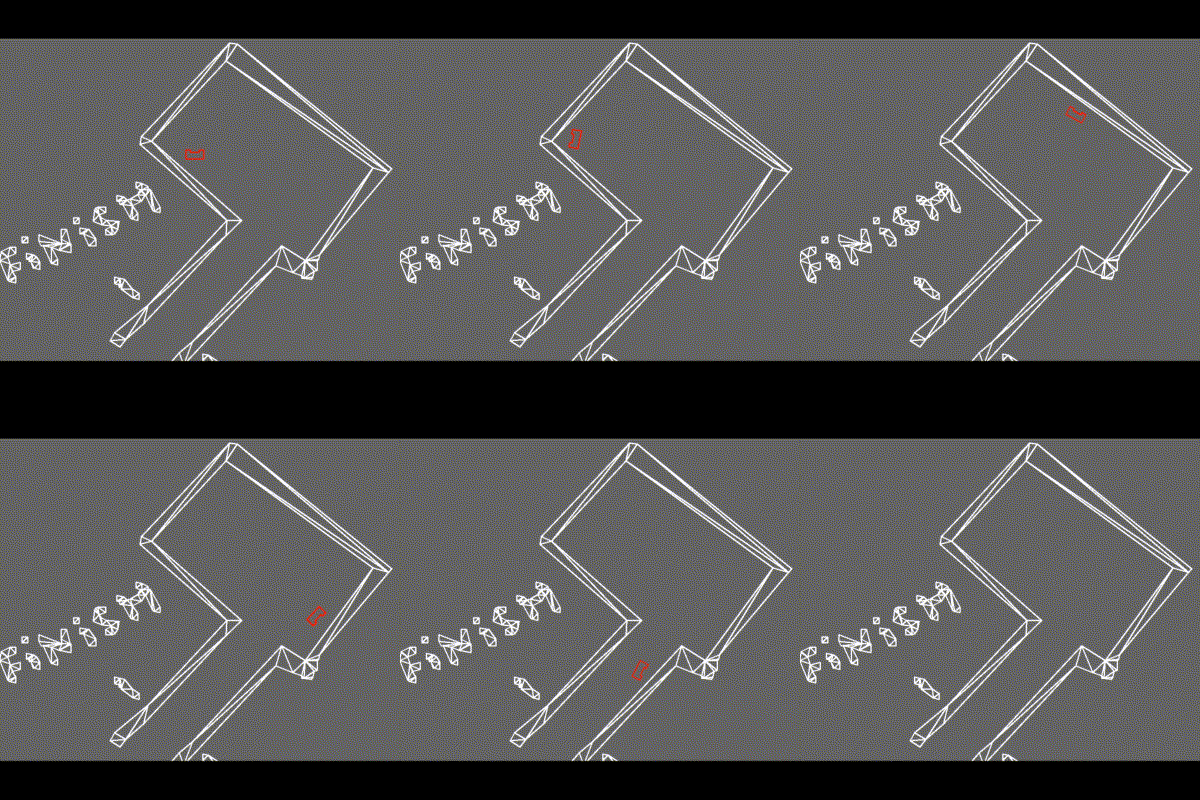
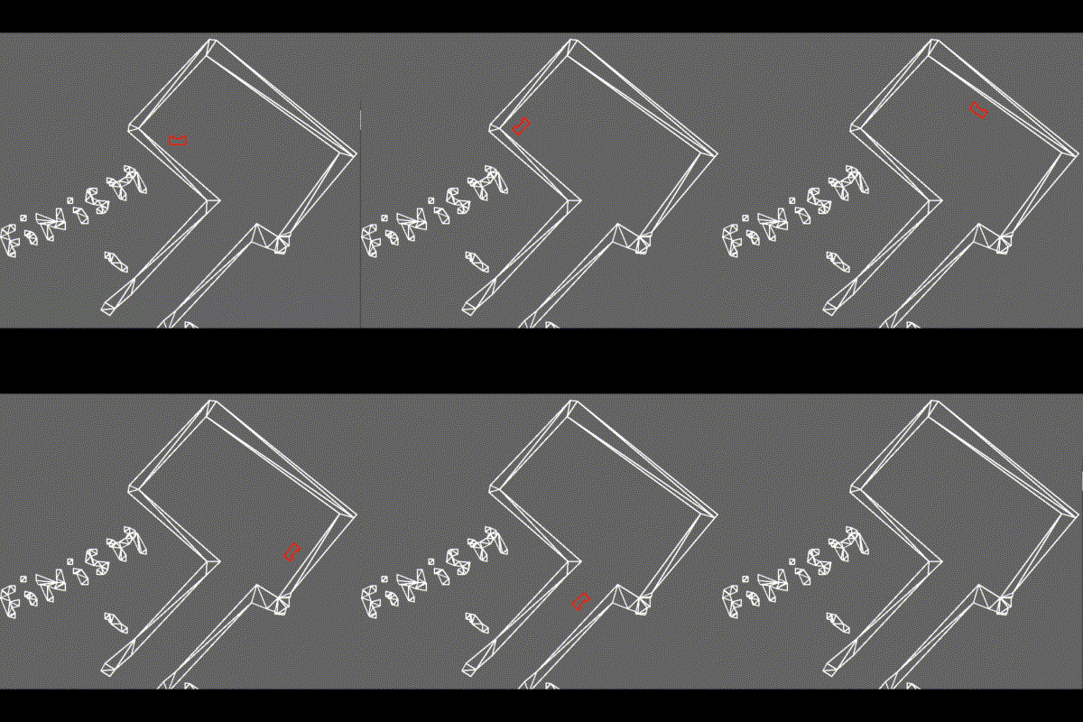
In the Escape Room Challenge, both the master code and the backup code was used. This section explains the performance of the master code, then highlights the difference in performance of the backup code. Note that the visualization below is not a recording of the Escape Room Challenge, but a new simulation using the same map.
Master
Initially, the robot performed its tasks as desired (as explained above). It satisfactorily found the closest wall, aligned itself, turned corners, and kept proper distance. Only when the robot was facing the exit did erroneous behavior occur. Instead of accurately identifying the exit, the robot believed it was facing a straight wall at a far distance. Thus it drove forward, attempting to maintain a constant distance to the wall. This caused it to clip through the wall with its left half, thereby failing the challenge.
The cause of this behavior has been identified as wheel slip. The robot sought to spot an exit (characterized by a reading of the laser range finder above a certain threshold) straight in front of it. Because the robot had slipped too far counter-clockwise, the range it found was within the threshold and therefore treated as a distant wall. Since the threshold was quite low, a slightly slanted wall or offset robot would not pose an issue, but the combination of both proved to be too much. This edge case could have been solved by searching for the exit in a forward-facing cone instead. Had this change been implemented, we are confident the code could reliably pass the Escape Room Challenge.
Backup
The backup option could not make an error in error detection, given the simple fact that it had no error detection in the first place. Since the robot made no fundamental distinction between inward-facing and outward-facing corners, it simply followed the wall into the exit corridor and cross the finish line.
HOSPITAL CHALLENGE
Requirements and Specifications


Software Structure
@everyone: This next part explains the software structure and needs to be put at the spot currently above the figure about software structure. ALSO THE FIGURE ON SOFTWARE STRUCTURE NEEDS TO BE UPDATED!
The figure below represents the general software structure that has been implemented for the hospital challenge. It has been based on the escape room challenge, where there are four main components. The first component is the brain, which takes in all the data from the other components, and based on that makes decisions on what to do next such as path planning. The next components are the eyes, which senses and stores the laser range data and odometry data of its surroundings. The third component are the legs, which performs the general actions of the robot such as moving through the environment. Finally, the last component is the world model. This model stores a version of the entire world map based on a .json file. In addition, it also stores a second version of the world model based on the position and laser data of the robot. This second map is used for updating and navigating the current model so that the robot knows where it is, where it needs to go and what it needs to do in order to reach it.

State Machine
TODO: @Roohi check if the state machine is complete
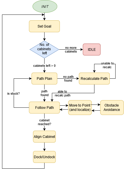
The state machine gives a general overview of the states the robot goes through in order to reach its goal, starting from the initial state. These states are described as the following.
Initialization
During initialization instances of all objects are made and are passed references to the objects they need to interact with as described in the software structure. Upon initialization, the world model reads in the provided JSON file to get the map without added obstacles and determine the location of all cabinets and reads in the cabinet order from the command line arguments in order to be able to provide the correct goal whenever requested. After all objects are initiated the brain starts in the initialization state, where it asks the world model to determine the initial position by doing a set of Montecarlo iterations of the localization algorithm in the starting area, and selecting the best result as the initial position. Having completed the initial localization the brain goes to the set goal state.
Localization
The way the robot is able to localize itself in its environment is by using a form of SLAM: Simultaneous Localization And Mapping. During the challenge, the robot will perceive its current surroundings by using its laser range finder. Using this laser data along with the map of the entire surrounding that has been provided, the robot will use an iterative closest point (ICP) algorithm to localize where it currently is based on the map. This algorithm first takes in the laser data as points, creating a point cloud. Then, for each of these points, the entire map is scanned to find which point on the map is the closest in distance to the current scanned point and is stored in a data set. Each element of this data set is then squared the results are summed up, creating a sum of squares of the total distance. The goal of ICP is to make this sum of squares as low as possible, resulting in most optimally all the scanned points being on top of a point in the given map, recreating a part of the map in terms of translation and rotation. If this total distance is too large, then a singular value decomposition (SVD) is performed. This SVD compares the orientations of the eigenvectors of the point cloud to the eigenvectors of the map and calculates a rotation and translation matrix needed to be applied in order to map both eigenvector sets on top of each other. This will cause the point current measured point cloud map to transform into an orientation that is more in line with the map, and therefore, reducing the total distance. Eventually, the total distance will be below a given maximum threshold, meaning that the current measurement fits a part of the map good enough, giving an identification of where the robot currently is.
It could be that this threshold is not reached after several iterations that has been set by the user. If that is the case, then the robot will give as output the final result, as this is its best attempt of locating its current position.
Set Goal
Set goal asks the world model what the next cabinet to go to is, print it to the pico speak, and make the state transition to "Find Path". If there is no next cabinet to go to it prints done to pico speak and transitions into the idle state.
Find Path
The find path state asks the world model for the position of the next goal and the current position of the robot. The accessible nodes are defined as the nodes that are at least 6 pixels or 4 pixels(used in backup code in which one pixel represents a larger distance) to the walls. Only the accessible nodes are used in the path plan. It then uses the A* algorithm to calculate a path from the current position to the goal and extracts only the turning points in order to only have strict movement to the most critical points in the path. The robot transitions to "Follow Path" from here.
The way to accelerate the computation is to design a reasonable heuristic function. The heuristic function used in this section is the distance between the goal and the considering node.
The A* algorithm is realized based on code from Justin Heyes-Jones. The Github link to his original code is https://github.com/justinhj/astar-algorithm-cpp.
Follow Path
Once the Path between the goal and the current position has been defined as a set of multiple targets, the task is to move between those target points in order to reach the goal, i.e. the cabinet. The next target according to the path so planned are stored in an array and indexed in order. We then move to the given target using the move to point algorithm. Once the target point is reached, i.e. the distance between the current position of the robot and the target point is within tolerance, the index is incremented to the next target point on the path. This is continued until the final goal is reached. Once the goal has been reached, we move to aligning with the cabinet.
Move to Point
The move to point algorithm operates in a fairly simple fashion. First, it converts the global Cartesian coordinates of its target point into local polar coordinates, relative to its own position. It will then rotate to face the point (within a certain tolerance), then drive forward until it has reached the point (within a certain tolerance). When it has reached the point the algorithm returns true, causing the follow path algorithm to send a new target point.
Align Cabinet
To start aligning the robot rotates to face the cabinet according to the localization and mapping, after that stage the robot works in closed-loop with the laser data in order to determine the position of the robot with respect to the cabinet without propagating the errors made in localization. For the closed-loop laser data feedback the robot uses the distance and angle to the closest point in a cone of 0.4 radians around the front of the robot. Firstly it checks whether the measured angle is more than a bound away from 0 since if the robot was aligned the angle would be 0 and rotates to get it within this bound. Secondly, it checks the minimum distance to see if the robot is not too close or too far from the cabinet, and move for- or backward to match the distance. The robot is tuned to stay 31 centimeters from the cabinet. Lastly, it checks the horizontal alignment by making sure the distance at the edges of our cone is similar to within a bound, and if that is not the case it moves sideways in the direction of the shortest distance until both hit the cabinet and are similar.
World Model
The world model is generated by reading in a json file. This json file contains a set of x and y coordinates, which are used to indicate the positions of the corners of walls, cabinets and the starting area, as wall as a set of lines that represents the walls and cabinets . Before the json file is read in, the vectors that will store these points and lines in the C++ file are emptied, which is done for the case when a new file has to be loaded in during the experiment. Once emptied, the points and lines from the previously named objects are stored in their corresponding vectors. Once it has stored these points, it creates a image of a size that is large enough to store in all coordinate points that have been stored in the vectors. This image is then converted to a grid map, and is made completely white. This grid map is then filled in by making the grids black that correspond to the lines and coordinates where the cabinets and walls are, based on the previously defined vectors. This results in the map of the current world model, which can be used for the robot to navigate through.

TODO : ICP images and writeup
Execution of the Hospital Challenge
TODO : @Gerben hospital challenge video execution with and without obstacles TODO : @Steven writeup
Code
In the end, the final program for the final hospital challenge was able to make the robot localize itself, recognize where its starting position was, and was able to plan a path to the correct goal starting from this position. In addition, the robot was also able to see and recognize obstructions that were on its path, and recalculated the path accordingly such that it would still be able to reach its goals. However, in general the performance of the robot could be improved at several points to speed it up. First, the robot took a long time to localize itself, due to the fact that the ICP algorithm takes quite some time to complete. At the beginning of the project, it was quickly decided to implement this algorithm, as it was a suitable candidate for both localization and map updating simultaneously and time was only limited. As a result, other algorithms were not really considered. For the future, if more time were to be spent on finding out the pros and cons of different localization algorithms, the team could decide which algorithm might be best suited for that current project.
Besides improving on localization, path planning itself could be improved. Right now, the path uses a grid-based algorithm, which results in the generation of many points on the map, that in the end will not be used for the current challenge. One way to improve this path planning algorithm, is to use a node-based path planning algorithm. Based on the map information and the current goal and position of the robot, this algorithm generates only a fixed set of nodes that are a specified Euclidean distance away from the each other. From this set of nodes, a path is drawn that is the shortest distance between the robot and its goal. Using this algorithm, by generating only a set of nodes that are a specific distance away from each other, less nodes need to be generated compared to the grid-based approach, meaning that the program only has to go over a smaller set of nodes, ultimately generating a path faster. This could be easily implemented in the current code, as the only things this algorithm requires is a start area, the most updated map and the current goal, all things which could be easily retrieved due to the way the code has been written. As a final note, the number of nodes that are generated are determined by the specified Euclidean size, which can be made smaller or larger, resulting in a higher or lower resolution of points. Of course, the current grid size could also be made less coarse in order to speed up the path finding algorithm.
One final thing that could be considered for improvement is the plan of approach that was taken for this project, which was based on working from milestone to milestone. For each milestone, there were a set of goals specified that needed to be reached before moving on to the next milestone. However, these milestones did not take future milestones into consideration. For example, when building the localization part of the program, it was built and optimized in an environment without obstacles. As a result, this feature was not optimal anymore in the next milestone when introducing obstacles, since it did not know how to deal with them. This came to our realization quite late in the project, and due to time constraints, was not added to the current plan of approach. Therefore, for future projects, it would be wise to also take future milestones into account when working on a certain milestone as this would save time that can be used for other parts in the project.