Embedded Motion Control 2019 Group 7

Group members

• Guus Bauwens - 0958439
• Ruben Beumer - 0967254
• Ainse Kokkelmans - 0957735
• Johan Kon - 0959920
• Koen de Vos - 0955647

Introduction

This wiki page describes the design process for the software as applied to the PICO robot within the context of the "Embedded Motion Control" course project. The project is comprised of two challenges: the escape room challenge and the hospital challenge. The goal of the escape room challenge is to exit the room autonomously as fast as possible. The goal of the hospital challenge is to autonomously visit an unknown number of cabinets as fast as possible.

Design Document

The design document, describing the initial design requirements, functions, components, specifications and interfaces, can be found here.

Challenge 1: The escape room

As an intermediate assignment, the PICO robot should autonomously escape a room through a door from any arbitrary initial position as fast as possible.

To complete this goal, the following steps are introduced:

1. The sensors and actuator are initialized.
2. From the initial position, the surroundings are scanned for gaps between the walls. If no openings are found, the robot is to rotate until the opening is within view.
3. The robot will drive towards a subtarget, placed at a small distance from the opening in order to avoid wall collisions.
4. Once arrived at the subtarget, the robot will rotate towards the target.
5. After being aligned with the target, the robot will drive straight trough the corridor.

To this end, methods for the detection of gaps between walls, the placement of (sub)targets and the path planning are required.

Gap detection

Scheme of a possible Escape Room, with PICO located in the upper left corner.

From the initial position, the surroundings are scanned using a Laser Range Finder (LFR). A gap is detected when there is a significant jump (of more than 0.4 [m]) between two subsequent data points. This method is chosen for its simplicity, it does not require any mapping or detection memory.

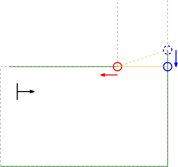
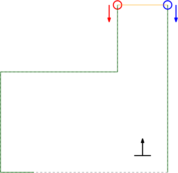
Within the context of the escape room challenge, either a one (from within the escape room) or two gaps (in front of or in the corridor) can be detected, as depicted in Figures \ref{} and \ref{}.

As can be seen in these Figures, dependent on PICO's orientation, gaps can be detected under an angle resulting in a false recognition of the corridor entry. To this end, the gap size is minimized by moving the points on the left and right side of the gap respectivily counterclockwise and clockwise. The result of this data processing is shown in the Figure \ref{} where the dotted orange line depicts the initial gap, and the straight orange line depicts the final gap. Here, the left (red) point is already optimal and the right (blue) point is optimized.

Scheme of a possible Escape Room, with PICO located in the lower right corner.

In this example of a possible situation, PICO is located straight in front of the corridor. In this case the gap cannot be optimized in the same way because moving either of the points increases the distance between the points (as they are not iterated at the same time). In Section xxx the script is expanded to deal with this scenario.

Dealing With Boundery Scenarios

Initially 2 detected data points are be expected, 1 of each corner of the exit. This would be the case if the escape rooms exit would have empty space behind it. Topology wise this is true, but in practice the LRF will possibly detect the back wall of the room the escaperoom is placed in or other obstructions standing around the exit.

In the case a (more or less solid) backwall is detected, the gap finder will find 2 gaps, one on each side of the exit. In this case point 1 and 4 are taken to determine the target. The target is defined as the midpoint between data points 1 and 4 and the subtarget is once again interpolated into the maze.

(Sub)Target Placement

As driving straight to the midpoint of an detected gap, will result in a collission with a wall in some circumstances, a subtarget is created. The target is interpolated into the escape room to a fixed distance perpendicular to the gap. This point is first targeted. PICO will turn that it is facing this point and will drive in a straight line to reach it. When PICO is approaching the subtarget, the corridor will become visible. As this removes the discontinuity in the data (as PICO can now see into the corridor), a new target is found consisting out of either 2 or 4 points. In the first case no backwall is detected, in the second case a back wall is detected. In this scenario two gaps will be found; to the left and to the right of the end of the exit. The new target will become the middle of the 1st and 4th point. A subtarget is possible, but will not change PICO's desired direction.

Path Planning

The loop of finding gaps is gone through continuously. The following cases are build in:

• 0 data points found

Protocol 1

If no data points are found, PICO should turn until it finds at least two data points. If not move to protocol 2.

Protocol 2

If after a full turn not data points were found, apparently no gaps are in range. PICO should move forward in a safe direction untill it either cannot move anymore, a maximum distance is reached, or data points are detected. If none are detected, return to protocol 1.

• 2 data points found

The 2 points are interpolated as target, the subtarget is interpolated. PICO should allign itself with the subtarget and move straight towards it.

• 4 data points found

Point 1 and 4 are interpolated as target, the subtarget is interpolated. PICO should allign itself with the subtarget and move straight towards it.

• > 4 datapoints found

In theory this should not happen. If so PICO should move forwards if this is safe to do so.

Dealing With Discontinuities In Walls

If a wall is not placed perfect, the LRF could find an obstruction behind the wall and indicate it as a gap (as the distance between the escape rooms wall and the obstruction will be bigger than the minimum value of a gap), while in practice the gap is way to small to fit through. These false positives should be filtered.

In the Figure to the right the algorithm used is presented. 4 points are detected as 2 jumps in data are detected. For convenience the points are numbered. The first point of every jump (the blue points) are checked for data points to the left that are too close by. If this is the case, the gap cannot be an exit. Likewise, the right (the red points) are checked for data too close by to the right.

Compare this to data points found in an actual gap. These points will never be to close by as the blue point will never have a data point to the left closer by then the minimum exit size (as will the red point to the left). Important to note is that this check is done with the initial gap detection data points, not with the optimized location. If it would, in this example the blue point of the actual exit has directly neighboring data to its left.

=== Dealing With Unwanted Discontinuities In LRF Data Mark data with no close neighbouring points as unvalid. ...

Challenge Review

We became second with a finish time of 60 seconds!

• Initially 2 doors where introduced in the escape room. PICO would not have been able to find the correct exit as no check was implemented for the extra requirement that the walls of the exit are 3 m. PICO would have driven to the exit it saw first. If both exits would have been seen at the same time, PICO should have chosen the closest one.

• Due to the long exit walls, PICO kept compensating its position in front of the exit. Buffers which should have limited this behavior where implemented, but due to the distance these where not sufficient. Also, due to the length of the exit the exit opening was closer to the obstacles around the RoboCup field, which partially messed up the non valid gap detection.

• During the first try PICO hit the wall, so the safe distance to a wall should be validated.

• Our lessons learned during the Escape room challenge are that we should
  • be more strict in how we interpreted world information.
  • not assume that certain scenarios (longer walls) work without testing

Challenge 2: Hospital (old)

State machine

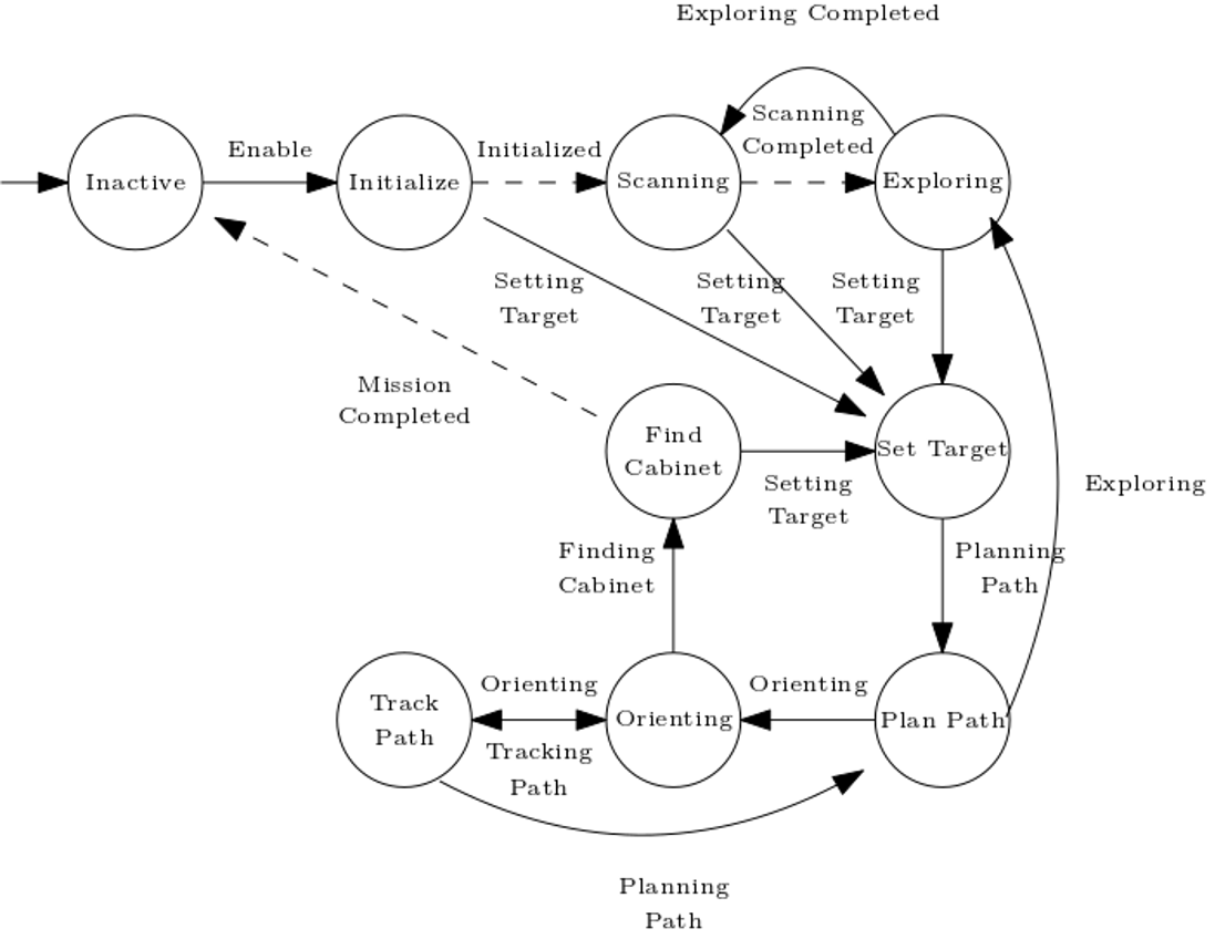
A finite state machine is designed as a means of sequential control logic, which forms the core of the system’s architecture. It allows for traversing through a predetermined sequence of states in an orderly fashion, facilitating the coordination of the implemented activities and behaviors.

Below a schematic overview of the state machine is depicted.

Low level control

controller, odometry, wall avoidance

Particle filter

The main goal of the particle filter is to estimate the pose (position and orientation) of PICO. In general, it holds that the more particles are used, the more accurate this estimate is. The disadvantage of using more particles is that the computations take more time, so the frequency with which the main loop can be executed becomes lower. This problem has (partly) been overcome by using a separate thread for the particle filter. This thread is executed simultaneously with the main loop, and can have a different update rate. The important data is shared using a mutex, which prevents that a variable would be read and/or written at two places in the code at the same time.

Static map

Given map with cabinets

Static obstacles

Doors and boxes. Doors are on locations that can be expected.

Dynamic obstacles

People

Path planning

A*

Obstacle avoidance

Once the path has been planned and is tracked by the feedforward and/or feedback controller, there still is a risk to hit a wall or obstacle. The path is planned based on the map and the tracking is done by means of the pose estimation from the particle filter. However, this pose estimation can and will have a small error, an obstacle could somehow not have been included in our (updated) map, etcetera. Therefore, a more direct approach is used as an extra safety means to avoid obstacles: potential fields.

The potential fields are based on only the most recent LRF data. In a small neighborhood around PICO, a local gridmap is made, with dots (the LRF data) that indicate where walls/obstacles are. This map is then converted to a field, in which the height is an indication of the distance from that point to its closest wall/obstacle. The scaled (discretized) gradient of this field is used as the actuation for the translational directions of PICO, to prevent collisions.

Using only the direct LRF-data for these potential fields also has a disadvantage: there is no data available in the region behind PICO. This problem is to a large extent overcome by not driving backwards.

Cabinet Detection

Make picture of data

Loading of the map

Converting to useful format

Challenge 2: Hospital (new)

Perception

The perception component is responsible for translating the output of the sensors, i.e. odometry data and LRF data, into conclusions on the position and enivorment of PICO.

Localization on the global map is performed using a particle filter. Detection of static obstacles is done using a histogram filter.

Monte Carlo Particle Filter (MCPF)

In the hosptial challenge it is very important that PICO is able to localize itself on the global map, which is provided before the start of the challenge. The particle filter is responsible for finding the starting location of PICO when the executable is started. After the initilization procedure it will keep monitoring and updating the position of PICO based on the available LRF and odometry data.

General Overview of implemented algorithm

• Initialization

When the excecutable is started PICO does not know where it is, besides being somewhere in the predefined starting area. In order to find the most likely starting position, or most likely starting position (more on this later), an initialization procedure was devised which is able to, whithin a limited time frame, find a set of possible starting positions. Finding this starting position is best described by the following pseudo code.

...
loop for N times
{
Intialize particles randomly
Calculate probability of particles
Pick and store X particles with largest probability
}
...

This algortihm provides the particle filter with a list of particles which describe the possible starting position of PICO. This list of particles is then used as an initial guess of the probability distribution which describes the location of PICO. This distribution is not necessarily unimodal, i.e. it is possible that a certain starting position delivers identical data with respect to another starting location. It is therefore not possible to immediately conclude that the mean of this distribution is the starting location of PICO. The probability distribution stored in the particle filter must first converge to a certain location, before the mean position can be send to the world model. Convergence of the probability distribution is tested by calculating the maximum distance between "likely" particles, in wich a "likely" particle is defined as a particle with a probability larger than a certain value. This distance is constantly monitored to determine wheter convergance has been achieved.

Often it is not possible for the particle filter to converge without additional information. This is for isntance the case when PICO is in a corner of a perfectly square room with no exit and perfectly straight corners. In this case the particle filter will first signal to the state machine that it has not yet converged, the state machine will then conclude that it has to start turning or exploring to provide the particle filter with extra information on the current location of PICO. When sufficient information has been collected to result in an unqiue location and orientation for PICO the particle filter will signal the state machine that it has converged. After convergence the particle filter will start its nominal operation, described below.

• Propagating on the basis of odometry data

• Find probability of certain particle
• Resample