Embedded Motion Control 2018 Group 2

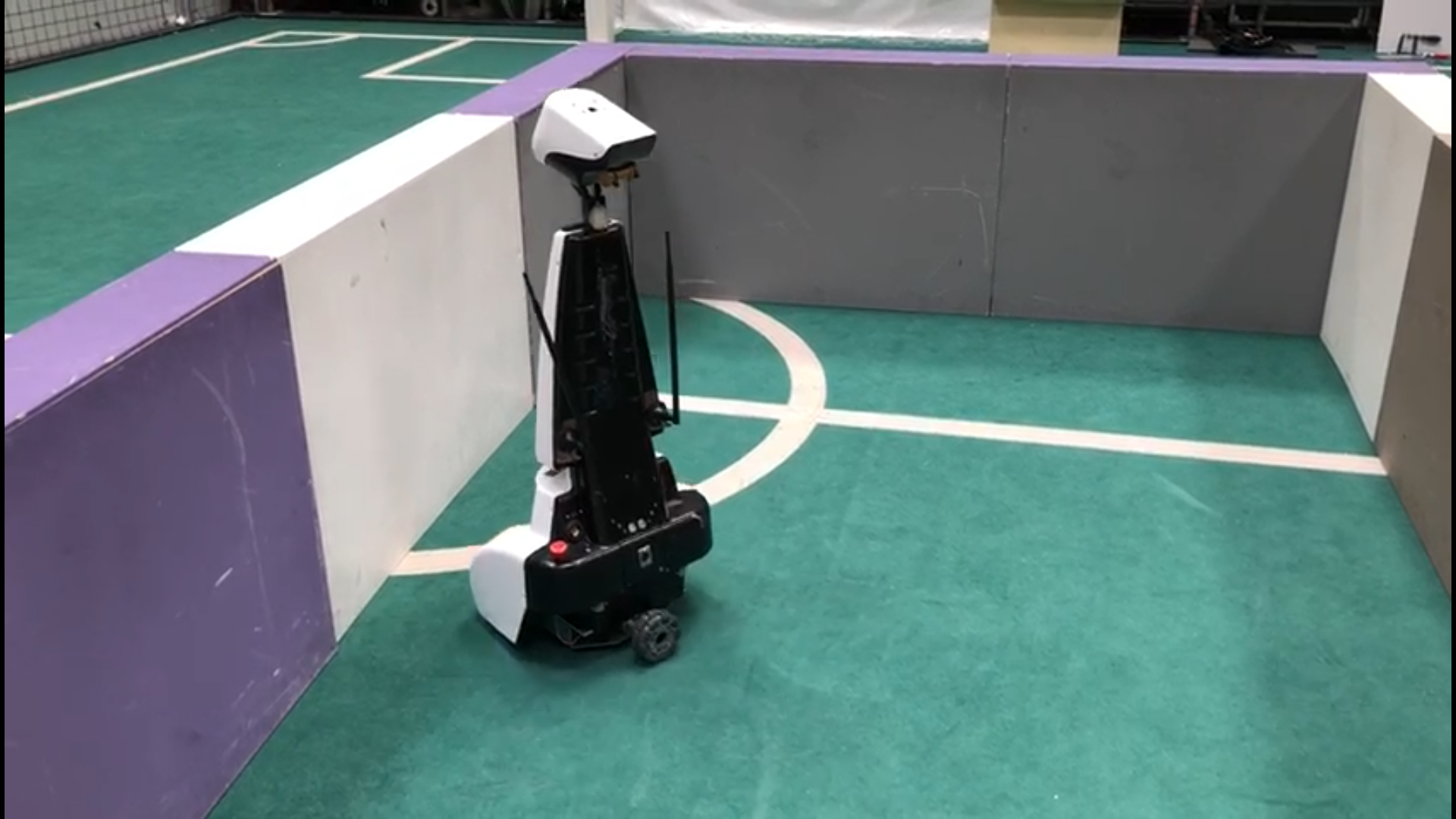
This wiki describes and explains the software that was made for and implemented on the PICO robot to complete this years Embedded Motion Control course. This year the course consists of two challenges, the escape room challenge and the hospital room challenge. Both these challenges will be discussed in more detail further down this wiki page. The robot that is used during the project is PICO. PICO has a holonomic wheelbase with which it can drive, a Laser Range Finder (LRF) from which it can gather information about the environment (blocked/free space) and wheels that are equipped with encoders to provide odometry data. Note that not all the software that is developed has to be tested solely on the robot, there is also a simulator available which provides an exact copy of PICO's functionalities. PICO itself has an on-board computer running Ubuntu 16.04. The programming language that is used during the course is C++ and Gitlab is used to store the code.

Group Members

TU/e Number	Name	E-mail
0843128	Robbert (R.) Louwers	r.louwers@student.tue.nl
1037038	Daniël (D.J.M.) Bos	D.J.M.Bos@student.tue.nl
0895324	Lars (L.G.L.) Janssen	l.g.l.janssen@student.tue.nl
1275801	Clara () Butt	clara.butt@aiesec.net
0848638	Dorus (D.) van Dinther	d.v.dinther@student.tue.nl

Relevant PDF Files

[|Initial Design Group 2]

[|Presentation Initial Design Group 2]

[| Presentation Final Design Group 2]

Motivation

Robotic systems become more and more important. At this stage, they are already used for montage processes, in logistics and many other fields. Creating stable autonomous behavior is the main difficulty while dealing with robots. As a mechanical engineer, it is a great advantage to know how to control a robotic system through an unknown environment.

Although our highest priority was, of course, to make the whole system working, it was important for us to learn as much as possible. Hence we decided to use tools like GMapping or different libraries but still tried to develop parts on our own. The potential field and path planning were some of them.

Initial Design

Introduction:

For the initial design, the requirements will be discussed as well as the functions and their specifications. Moreover, a list of possible components and a suiting interface is designed.

Note that this is an initial design towards the hospital competition which has overlap with the escape room competition. Some distinction will be indicated.

Requirements:

• Execute all tasks autonomously.
• Perform all tasks without bumping into a wall.
• Perform all tasks without getting stuck in a loop.
• Finish both challenges as fast as possible, but at most within 5 minutes.
• Escape room competition:
  • Locate the exit and leave the room through this exit.
  • Keep a minimum distance of 20 cm to the walls or any other objects.
• Final competition:
  • Explore and map the hospital rooms.
  • Use the map to get back to the starting position and park backwards into the wall behind it using both the map and the control effort.
  • Use a map to find and stop next to the object that is placed in one of the rooms after the first

• Nice to have: Use the provided hint to be able to find the placed object directly without searching.

Functions:

he functions that are going to be implemented are subdivided into three different types of functionality. First of all, there is the lowest level functionality, which will be referred to as the motion functions. These functions will be used to interact directly with the robot. This interaction will be specified more precisely in the function overview that can be found below. The mid-level functionality, which will be referred to as the skill functions. As the name mid-level functionality already suggests these functions act on a more abstract level and are built to be able to perform a specific action. All the actions that will be implemented in the skill functions can also be seen in the overview below. Finally, there is the high-level functionality, which will be referred to as task functions. These functions are the most abstract and are structured to carry out a specific task, which consists of multiple actions.

To give a full overview: in a task function, a specific order of actions will be specified in order to be able to fulfill the task. The actions that the robot can perform, and are therefore available to be called by the task functions, are specified in the skill functions. The motion functions are used in the skill functions to be able to invoke physical behavior by the robot.

• Motion functions
  • Actuation: Using the actuation function PICO is given the command to drive in a specific direction or to turn in a specific direction. The input to this function is a movement vector which specifies in which direction and how far the robot should move. The output is actual robot movement according to this vector and the control effort needed for this movement.
  • Obtain information: Using the obtain information function sensor readings can be requested. The input for this function is the request of a (sub)set of sensor data from a specific sensor(set), either the Laser Range Finder (LRF) or the odometry encoders.

• Skill functions
  • Path planning: Using the path planning function a (set of) movement vectors is defined on the basis of the map to reach the defined goal. The input for this function is the current map and the goal that should be reached. The output of this function is a (set of) movement vectors.
  • Object avoidance: Using the object avoidance function it is ensured that PICO does not hit any objects. The input for this function is the LRF sensor data and the movement vector. If the movement vector prescribes a movement that collides with an object that is detected by the LRF the movement vector is adjusted such that PICO keeps a safe distance from the object. The output of this function is, therefore, an (adjusted) movement vector.
  • Mapping and localization: Using the mapping and localization skill a map of the environment is built up and PICO's location in this environment is determined. The input for this function is sensor information and actuation information that can be obtained from the motion functions. Using the LRF data PICO's environment can be defined in "blocked" and "free" area's, places in which obstacles are present and absent respectively. Using the odometry encoders and the control effort the location of PICO can be tracked in the environment. The output of this function is a visual map, that is expanded and updated every time this function is called.
  • Semantic mapping: Using the semantic mapping function extra information is added to the basic environment map. This function has as input the basic environment map. The surface of this map will be split into different sections which can have one of two different types of identifiers assigned to them: room or hallway. Both the splitting of the sections and the identifications of the sections will be based on shape fitting. If a rectangular shape can be fitted over (a piece of) the basic map, based on the LRF, this (piece of the) map will be defined a (separate) section with the identifier room. Note that each section with the identifier room will be given a separate number to be able to distinguish the different rooms from each other. This is necessary in order to be able to use the hint that will be given for the final challenge. The output of this function is a visual semantic map that is updated every time this function is called.

• Task functions
  • Exit a mapped room: This is the escape room challenge. In this task, all motion skills and all skill functions, except the semantic mapping skill, will be used.
  • Semantically map an entire floor and return to the beginning position: This is the first part of the final challenge. In this task, all motion and skills functions will be called.
  • Find an item in the semantically mapped floor, preferably using the provided hint on the position of the item: This is the second part of the final challenge. In this task again all motion skills will be used and all the skill functions except the semantic mapping skill.

Components:

To be able to execute the challenges the PICO robot, already mentioned above, will be used. The following hardware components will be utilized:

• Actuators:
  • Holonomic base with three omni-wheels.
• Sensors:
  • Laser range finder (LRF): To detect the distances to objects in the environment.
    • Range: To be determined
    • Field of view: 270 degrees
    • Accuracy: To be determined
  • Wheel encoders: Combined with the control effort these encoders keep track of the robot's position relative to its starting point. (This has to be double checked with the position in the map since the encoders easily accumulate errors.)
    • Accuracy: To be determined
• Computer
  • Running Ubuntu 16.04.

Specifications:

The specifications are based on the requirements.

• The maximal transitional velocity of PICO in any direction is 0.5 [m/s].
• The maximal rotational velocity of PICO is limited to 1.2 [rad/s]
• PICO should not stand still or make no sensible movements for periods over 30 [seconds].
• Escape room competition:
  • PICO has to finish the Escape Room within 5 [min].
  • The width of the corridor and the openings in the walls are between 0.5 [m] and 1.5 [m].
  • The shape of the room is rectangular.
  • The exit is located more than 3 [m] into the corridor.
• Hospital competition:
  • PICO has to finish the Hospital within 5 [min].
  • The width of the corridor and the openings in the walls are between 0.5 [m] and 1.5 [m].

The first interface:

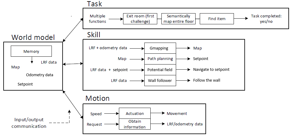
The interfaces describe the data that is communicated between the several parts of code that will be developed. The functions that are discussed in the Chapter Functions are all part of the interface, however, there is one other important piece in this interface: the world model. The world model will contain the most recent (semantic) environment map with the location of PICO included in it. The motion, skill and task functions can monitor and request the information that is stored in this world model and use it to properly execute their function. A graphic showing the interface between the world model and the tasks, skills, and motions is shown below.

Figure 1: The first interfaces

The final interface:

While progressing through the project, a number of circumstances and insights gave reason to re-think certain parts of the initial design, which were altered accordingly. The requirements, components, and specifications have not changed drastically, only small updates have been done to address missing information. These parts will therefore not be addressed. The functions and therefore the interface, however, have been changed quite a lot.

To start off the functions will be discussed. First of all the motion functions. In the motion functions, the actuation has been implemented a little differently than specified above. It has been simplified such that as an input to this function the desired speed in a certain direction is given, so the robot can only drive in one of the directions (x, y or theta) at a time. The output of this functions is actual robot movement, but next to this, using odometry data, also the driven distance is given as an output. Note that there are two changes to the initial design, first of all, the initial design specifies the distance and not velocity and secondly the initial design specifies a vector and not a single turning direction. The first change was a forced change since the base of PICO only takes velocity as an input, not distance. The second change was a choice, to prevent slip it was chosen to only drive in one direction at a time. The second function within the motion functions, the obtain information function, was not needed since this functionality was already provided in the emc framework.

Secondly the skill functions. The skill functions have changed very drastically. The main reason for this lies in the fact that these relatively elegant and complicated functions could not be made due to the time limitations and lack of programming experience. Therefore a less complicated and more task specified structure has been used.

The first thing to note about the skill functions is the fact that in the initial design a specific feature is missing, namely the setting of a goal. This is not specified anywhere. In the final design, it is chosen to implement this part in the path planning. The rest of the path planning function has also been changed. Now the complete map, so the map of the whole driving area (so the room and the hospital floor respectively for the challenges), is given as an input for the path planning, while the output is a set of coordinates that PICO has to drive to. Note that the movement vectors have been completely left out. The choice to use the complete map instead of using map parts to set a target reduces the effectivity of the robot quite drastically since now no ‘smart decisions’ can be made. However, this choice is very much needed since the implementation of these ‘smart decisions’ is very difficult in an environment with so much unknowns. However, if these unknowns can first be mapped then it gets a whole lot easier to make these decisions. Thus the path planning has been implemented in this way to make the choices the robot has to make a lot easier and therefore hopefully more robust. Note that the name path planning is a bit misleading, it is more like target setting, however, the name that was used and is therefore presented here is path planning.

In order to be able to give this complete map of the world to the path planning function, there are two necessary functionalities. First of all the mapping, which makes said map, and some kind of driving function that makes sure that the complete environment is mapped. The easiest option for this kind of functionality is to use a combination of the mapping function, which has been proposed in the initial design, and a new function which follows the walls of the environment. Given the lasers specifications and the fact that it is known that the final challenge is performed a closed environment, this combination assures that the whole environment has been mapped. This new wall following function takes as an input the laser and odometry data and gives as an output robot movement. The specific implementation of this function can be found below, as holds for the other functions as well. Note that this wall follower returns roughly to the initial position, but not exactly.

Now that the complete navigation has been discussed the proposed object avoidance function can be discussed. The new implementation of the navigation causes problems in the proposed object avoidance function. To solve these problems and a the same time make the object avoidance safer the new object avoidance uses as the input the laser data and gives as the output a “force”, implemented in movement, that keeps PICO at least a certain distance from the wall. Note that the combination of using the path planning and the object avoidance can lead to deadlock situations, so this has to be handled with extreme care.

The only function that has not been changed with respect to the initial design is the mapping function. Since this function is not changed, nothing more will be said about it here.

The last function that was proposed in the initial design was the semantic mapping function. Due to the previously mentioned changes and the nature of tip that was provided on the location of the object the described semantic mapping function was no longer necessary. This function was therefore omitted completely. The relevant piece of semantic mapping, the detecting of the doors, was moved to the path planning (target setting) function.

The task functions were changed according to the changes in the skill functions as described above. Using these new or updated functions the final interface was made. This interface can be seen below.

Figure 2: The final interfaces

Using the given functions the following approach will be used to try and finish the final challenge:

• The wall follower function, in combination with the mapping function, will be used to map the entire floor and roughly get back to the initial position.
• Using some functionality that is specified in the state machine, so not in one of the functions, PICO, will drive backwards into a predetermined wall. Note that this functionality is discussed below.
• Using the path planning function, the object avoidance function and the high-level tip PICO will move to the room in which the object is located.
• Using another state machine based functionality that will be described below and the mapping function PICO will locate the object and stop near this object.

The Escape Room Challenge

The first challenge that had to be completed was the Escape Room Challenge. In this challenge, PICO had to escape from a room with a single exit.

Wall follower

The method that was chosen to let PICO complete the Escape Room Challenge was through a wall follower. This wall follower uses three beams to check if there is free space in front, and on its sides. Figure 3 shows these beams.

Figure 3: Space recognition beams (http://cstwiki.wtb.tue.nl/index.php?title=Embedded_Motion_Control_2017_Group_4)

The idea for this method of driving around was obtained from the Wiki page of Group 4 of Embedded Motion Control 2017.

Whenever the beam in front does not see any obstacles, PICO will drive forward. If an obstacle is seen in front, but the space to the right is free, then PICO will turn right. After making its right turn, PICO will start driving forward again. When the front and right are blocked, but the left is free, then PICO will turn left. If the front, left and right are all blocked, PICO will turn around and drive back the way it came, searching for an exit somewhere else. A video of PICO driving around using the wall follower is available by clicking the link below.

Sadly, this wall follower did not work yet at the time of the Escape Room Challenge, so PICO was not able to escape the room. However, shortly after the challenge, the wall follower did work and an improved version of it will be used in the Hospital challenge.

The Hospital Challenge

The second challenge of this course is the Hospital Challenge. In this challenge, PICO first has to drive around the hospital floor and map its environment. When the mapping is done, PICO has to drive back to its starting point and park backwards into the wall. In the second part of the challenge, PICO has to find an object that is placed somewhere on the hospital floor after the first part of the challenge is completed. The software components that were developed to complete this challenge are described below.

Mapping & Localization

The necessity of mapping in the hospital challenge is of two-fold. First of all, a map is necessary to be able to detect the new object that will be placed in the environment after the initial mapping round. The new object can be found by comparing the map with the current environment. The second reason a map is needed is for the navigation purposes. In the final challenge navigation through rooms and hallways is needed to be able to get to the newly placed object. To be able to perform this navigation task certain knowledge of the rooms, hallways and walls need to be stored, since this knowledge is needed for calculations that for example lead to the path planning. What information needs to be stored and in what format this information needs to depend on the task at hand. For the hospital challenge, a simple grid with "blocked" and "free" squares suffices.

However to be able to perform navigation not only information about the environment is important, the position of PICO itself is also important. There are different ways in which this localization of PICO can be done, however, not all options are equally robust or suited for the task at hand. One of the options that can be used to track the position of PICO is to use the encoders of the wheels, referred to as odometry data. Using this odometry data is however not very accurate for determining the position of the robot in the long run since the position errors, for example, caused by slip, integrate over time. To increase the accuracy of the localization of the robot often other sensor data is used in combination with this odometry data.

Figure 2: Transform setup for gmapping

The mapping and the localization problem can be tackled simultaneously by a method called SLAM (Simultaneous Localization And Mapping). There are other methods that solve these problems one by one, but in robotics, SLAM is an often used and proven method. In the SLAM method, there are again different techniques to obtain the desired result. Some popular techniques include the particle filter, extended Kalman filter, and GraphSLAM. The method that is best fit to solve the SLAM problem depends on the available resources and the requirements, which again depend on the task description. Given the available resources for the hospital challenge, there are still quite a few different possible SLAM algorithms that can be implemented. Some specific research was done into Extended Kalman Filter based SLAM (EKF SLAM) and particle filter SLAM. It was found that particle filter based SLAM has some advantages over EKF based SLAM, especially in dealing with non-linearities. Furthermore, particle filter based SLAM is robust to ambiguities in data association which can also be an advantage.

The Robot Operation System (ROS) that runs under the hood of the provided emc-environment provides a highly efficient Rao-Blackwellized particle filer under the name gmapping [3]. In this particle filter, all particles carry an individual map of the world. The number of particles is reduced by taking into account the movement of the robot, the odometry data, and the most recent observation of the environment, the laser range data. This method results in a 2-D occupancy grid map. One specific feature of this gmapping algorithm, which is not specifically necessary for the hospital challenge but very useful for real-world applications, is the loop closing feature. In loop closing the current environment is matched with previously mapped environments to track whether to mapping entity has returned to a previously visited location, possibly through an alternative route. This feature allows for accurate mapping of loops.

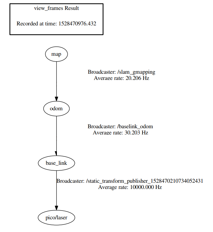
As mentioned above the input for this slam_gmapping node exists of the laser range data and the odometry data that are collected by PICO. However, this is not enough to be able to create the desired floor plan with occupancy information. What more is needed are the real-time transformations between different coordinate frames. This is necessary since the obtained data, the laser data and the odometry data, are collected in different coordinate frames. So in order for the gmapping algorithm to be able to function properly two coordinate frame transforms are needed. The first transform is between the laser range finder and the base of PICO (base_link -> /pico/laser). This transform is static since the laser range finder is physically attached to the base of the robot. The second transform is between the base of the robot and the initial position of the robot (odom -> base_link). This is a dynamic transform. Using these two transformations the gmapping algorithm makes another transform, namely the one from the initial position of the robot to the map. A graphical representation of this transform tree can be seen on the right side.

The above-mentioned transforms were not implemented on PICO by default, so they had to be created. To make the dynamic transform between the initial position of the robot and the base of the robot the odometry data is used. This odometry data, that was read out from the corresponding rostopic using a subscriber, was transformed into the right type and broadcasted to the tf topic using a tf broadcaster. The static transform between the laser range finder and the position of the robot is a lot simpler. This static transform is made using a single command that describes the absolute position of the laser range finder with respect to the center of the base of PICO.

Now all components are available gmapping can be called. This can again be done using a single command. In this command, a lot of parameters can be set. The most important parameter is the one that defines on which rostopic gmapping can find the laser data of the robot, which is in this case /pico/laser. The other parameters that have been altered from the default value are the max_range of the laser, the map update interval, the dimensions of the map and the map resolution. All these parameters have been altered to the goal of limiting the amount of data that is transferred without losing accuracy.

Since the update time of the map can be altered the map can be visualized nearly real-time. This near real-time visualization can be performed in a program called Rviz. This program not only shows the map of the environment but also shows PICO's position which is a very handy tool to use for testing.

All in all to run this gmapping algorithm quite a few commands have to be given in different terminals. To simplify this process a bash shell has been made that gives all of these commands at once when the shell is executed.

Wall Follower

For the first part of the Hospital Challenge, which consists of PICO driving around, mapping the floor and parking at its starting position, again a wall follower is used. This wall follower is similar to the wall follower that was planned to use during the Escape Room challenge which was explained above. However, the wall follower now also makes use of the potential field in order to move the robot. More details on the exact workings of the potential field can be found further down the wiki.

Using the wall follower instead of directly sending a speed for PICO makes movement a lot safer, in the sense that it is highly unlikely to bump into walls using the potential field algorithm. The previous version was not robust enough so that it would never hit a corner. Other than bumping protection, the potential field makes it easier to program the structure in such a way that PICO does not deviate from the wall on the right that it is following. This is done by making PICO move slightly northwest, rather than simply moving north. The potential field then ensures that it moves straight along the wall due to the repulsive forces.

The logic that is used to guide PICO around the floor is similar to the section on Space Recognition in the Escape Room Challenge. A more detailed description of the final state-machine switches is as follows:

• It first moves to the right until PICO finds a wall on its right, then switches to moving forward
• While moving forward it can either turn right or turn left. It turns left if there is a wall at the top of PICO and goes to the turn_right state if there is free space on the right.
• When turning left, it turns until it has turned approximately 90 degrees counter-clockwise, then goes back to driving forward.
• Turning right is a more complex state. Since the wall follower is a right-hand wall follower, it has to follow the wall on the right along right corners. In order to achieve this, PICO moves forward a bit (based on gmapping localization data) and then turns around approximately 90 degrees clockwise and moves forward a bit again until it has found a wall on its right, after which the state switches back to moving forward.

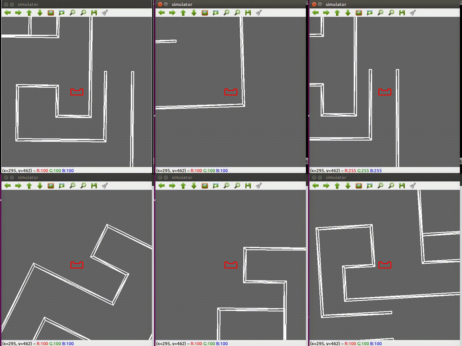
When the location of PICO is close enough to its starting point (taken as an absolute distance in the sense of [math]\displaystyle{ \sqrt{x^2 + y^2} }[/math]), it will switch to its parking state. The GIF below shows the wall follower in action. In the final seconds of the GIF, the parking state is demonstrated. In this case, PICO does not drive backward into a wall but instead drives back a set distance, because there is no control effort in the simulator.

Moreover, there are a number of fail-safes implemented to keep it from getting stuck in a loop (mainly the turning right state), by either going back to driving forward or finding a wall in certain situations. However, as with most fail-safes, these should not actually be needed if the wall follower does its job correctly.

Parking

For parking, there are again multiple alternatives that were investigated and thought about. One way is to base the parking on the gmapping data, from which to the location of the back wall and PICO can be retrieved. However, it is not a sufficiently robust method since there might be inaccuracies in PICO's location, the location of the back wall or maybe even which wall is defined as the back wall. Moreover, the current map has a 10 [cm] resolution which is not detailed enough to determine the wall location which is important on an approximately 1 [cm] scale. Increasing the resolution (without decreasing the map size) would lead to a bigger occupancy grid matrix, which would really only be necessary for the parking. A similar method involves using the laser data in combination with the odometry data. However, this is even more inaccurate, mainly because of the odometry data. These methods would both overcomplicate the matter more than necessary, which is why we chose to base the method on the control effort of the odometry wheels, as described below.

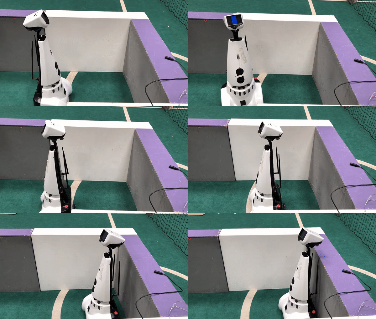
After the state-machine switches from the wall-follower to parking as explained in the previous section, its objective is to park backwards into a wall and shout "I am parked!". This is done by first turning PICO 180 degrees as it is assumed that PICO arrives in the parking state facing the back wall which it should park back into.

After turning, it moves backwards at a fifth of its maximum speed until the absolute control effort in x-direction reaches a limit of 440. This limit has been found by calling the control effort when PICO was driving backwards into a wall during testing. Moreover, an extra fail-safe is implemented, which guarantees that PICO stops moving backwards if it has moved more than 1.3 [m] after turning (based on odometry data). The challenge describes that the back wall is a maximum of 1 [m] from PICO's initial location, so including slip, PICO should still stop driving backwards even if the control effort condition is not met (bigger than 440).

After it bumps into a wall, the movement of PICO is stopped and PICO shouts "Boom is ho, I am parked!". This also ends the first part of the challenge. The second part of the challenge is planned to be solved using a path planning, potential field, and object recognition algorithm as described in the following sections.

Object avoidance

The potential field algorithm makes sure that PICO does not run into any walls (or anything else for that matter). As an input, it requires a movement direction in which the PICO should move using the coordinate frame in Figure 4. As an output, it provides an altered speed vector which can be sent to PICO. It works by balancing attractive forces in the movement direction of PICO with the repulsive forces generated when the laser detects something in a range. An interpretation of the algorithm is shown in Figure 4. The structure is based on the same structure used by Group 2 of last year.

Some of the reasons for choosing this algorithm is that it was proven successful by previous years. Moreover, it can make the path planning algorithm a lot easier, because when using this potential field algorithm, the path planning does not have to take care of running into a wall and can simply provide a movement setpoint for PICO.

Figure 4: Graphic interpretation of potential field.

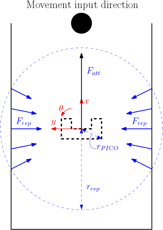
First of all, the attraction force is calculated by calculating the magnitude of the attraction force in the setpoint direction [math]\displaystyle{ (s_x, s_y) }[/math] as

[math]\displaystyle{ r_{att} = F_{good} \sqrt{s_x^2 + s_y^2} }[/math]

and then the angle [rad] at which the setpoint vector is positioned through

[math]\displaystyle{ a_{att} = \arctan \left( \frac{s_y}{s_x} \right) }[/math]

Note that the math.h package is used for certain operations in C++, including the 4-quadrant arctan function "atan2". The magnitude [math]\displaystyle{ r_{att} }[/math] and angle [math]\displaystyle{ a_{att} }[/math] form a polar coordinate frame, which is converted back to the cartesian PICO frame by

[math]\displaystyle{ F_{att} = \begin{bmatrix} F_{att,x} \\ F_{att,y} \end{bmatrix} = \begin{bmatrix} r_{att} \cos(a_{att}) \\ r_{att} \sin(a_{att}) \end{bmatrix} }[/math]

Similarly, the repulsive forces are calculated by converting the filtered laser data (distance [math]\displaystyle{ r }[/math] in [m], angle [math]\displaystyle{ \theta }[/math] in [rad]) to cartesian coordinates. The filtered laser data is the original laser data with an extra row indicating whether or not a scan entry is bigger or smaller than 0.15 (sees itself). Moreover, only data is considered within a range of 0.6 [m]. The magnitude of the repulsive forces for each angle increment of the filtered LRF data is then calculated as follows

[math]\displaystyle{ r_{rep}(i) = \frac{-F_{bad}}{\left(\sqrt{\left( (r(i) - r_{PICO}) \cos(\theta(i)) \right)^2 + \left( (r(i) - r_{PICO}) \sin(\theta(i)) \right)^2}\right)^3} }[/math]

Note that the term [math]\displaystyle{ (r - r_{PICO} }[/math] is used instead of simply using [math]\displaystyle{ r }[/math], such that the denominator of the above equation goes to zero if PICO gets close to the walls. If the scaling with [math]\displaystyle{ r_{PICO} }[/math] had not been applied, then the magnitude would not go to infinity if PICO gets close to a wall. The extra power 3 is simply added to increase the repulsive forces faster if PICO gets close to a wall. The repulsive forces in cartesian coordinates are then calculated with

[math]\displaystyle{ F_{rep} = \begin{bmatrix} F_{rep,x} \\ F_{rep,y} \end{bmatrix} = \sum_{i} \begin{bmatrix} r_{rep}(i) \cos(\theta(i)) \\ r_{rep}(i) \sin(\theta(i)) \end{bmatrix} }[/math]

With both the repulsive forces and attraction forces, the total force can be calculated as

[math]\displaystyle{ F_{tot} = F_{att} + F_{rep} }[/math]

which is then used to determine the speed at which the robot should move as follows

[math]\displaystyle{ v_{PICO} = \begin{bmatrix} v_x \\ v_y \\ v_{\theta} \end{bmatrix} = \begin{bmatrix} F_{tot,x} \\ F_{tot,y} \\ \frac{1}{\theta_{sc}} \arctan \left( \frac{F_{tot,x}}{F_{tot,y}} \right) \end{bmatrix} }[/math]

where [math]\displaystyle{ \theta_{sc} }[/math] is a scaling constant to limit rotational speed. Moreover, the values in the speed vector are clipped such that they are bounded by the physical limits of the robot:

• [math]\displaystyle{ v_x }[/math] by [math]\displaystyle{ \pm 0.5/n }[/math] [m/s]
• [math]\displaystyle{ v_y }[/math] by [math]\displaystyle{ \pm 0.5/n }[/math] [m/s]
• [math]\displaystyle{ v_\theta }[/math] by [math]\displaystyle{ \pm 1.2/n }[/math] [rad/s]

where n is a scaling constant which can limit the speed even more during testing.

In short:

The repulsive forces go to infinity if the robot gets close to the wall and are therefore dominant in [math]\displaystyle{ F_{tot} }[/math] close to walls. If PICO is further away from the walls then the repulsive forces are negligent and the speed vector moves PICO to the movement direction of the input.

Note that this algorithm obviously cannot detect anything outside the LRF range of approximately 270 degrees. This means that if the robot moves backwards into a corner it will hit the corner and maybe also hit a wall if it drives backwards into a wall. To prevent this from happening, a fail-safe is implemented which prevents PICO from moving backwards, which works by only allowing PICO to turn if the movement vector is aimed at PICO's back area.

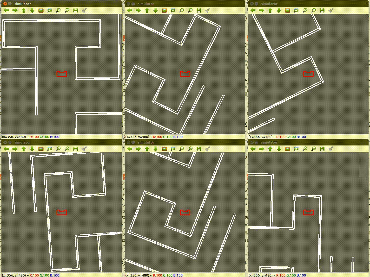
Below is a GIF showing the potential field working with a constant setpoint in the positive x-direction: (1,0). The repelling forces send PICO away from walls and the attractive forces are in this case constant in the (1,0) setpoint direction.

Path Planning

The path planning can be divided into three main parts:

- Semantic mapping

- Local target setting

- Global target setting

Semantic mapping

In the first part, the map has to be evaluated semantically.

The output of GMapping is an occupancy grid, a 400x400 matrix filled with zeros for unoccupied space, a minus one for unknown space and a value higher than zero for occupied space. The origin of the coordinate system of the map lays in the middle and goes from minus twenty to twenty meters. So the resolution of the matrix is ten centimeters.

The goal of our semantic map is to identify doors and assign them to two rooms.

As a first step, it has to be clear which parts of the map build a room. The second is to identify the edges of all doors in the room. Last, but not least the middle of each door has to be found and given as a target point for the robot. Furthermore, it has to be clear which parts of the map already have been scanned.

Store room

To accomplish step one the program goes through the lines of the occupancy grid until it finds an unoccupied element. From there it saves all unoccupied elements in the line until it hits an occupied one. It saves the data as a line in the room and sets the current position at the end of the first line in the room. After that, it goes through all lines of the room and saves them after the same scheme. All scanned elements are marked as scanned.

Identify door edges

Is the program done scanning all lines of the room, it starts searching for the lines with the largest difference in length compared to their neighbors. Has a line compared to its neighbors a much larger number of elements, it has to be part of more than one room and marks a door. This difference cannot be explained in another way.

Right after the program has found the line of the edge, it can search for an edge point. Therefore it first has to know if the door is on the right or left side of the room. It compares the first and last element of the current and the previous line. It checks, on which side the difference in column number is larger.

A problem might occur, when two edges are included in one line, one on each side of the room. It can be solved by checking if both sides of the line differ more than a maximally allowed difference from their neighbors first and last element.

Is clear on which side the edge is located, the coordinates have to be set. The x-position (line number) of the edge was already identified. Is the door on the left side of the room, the y-position (column number) is set as the column number of the first element in the compared row. Is it on the right side, the last element of the compared row is taken.

Exceptions

Is one side of the door part of the wall, the program cannot detect it in the previously described way. In this case, the program analyses on which side of the first recognized edge line numbers are larger. It scans the elements on the larger side until it hits the wall and saves the wall as a second door edge.

Identify middle of door and create target

Are two edges found, that belong to one door, the middle of the door and the target point is determined by the average of the line and column numbers of both edges.

[math]\displaystyle{ r_{middle,x} = \left( \frac{r_{edge1,x}+r_{edge2,x}}{2} \right) }[/math] , [math]\displaystyle{ r_{middle,y} = \left( \frac{r_{edge1,y}+r_{edge2,y}}{2} \right) }[/math]

Local target

The local target, the target the robot has to reach next, is always the middle of a door. In order to give the robot a proper target vector, first, the vector from the robot to the target has to be built in the coordinate system the map is built in.

[math]\displaystyle{ r_{t0} = r_{t0,room}- r_{t0,robot} }[/math]

After that, the vector has to be transformed to the coordinate system of the robot. This can be reached by using the transformation matrix for turning around the z-axis.

[math]\displaystyle{ r_tr = \begin{bmatrix} r_{tr,x} \\ r_{tr,y} \end{bmatrix} = \begin{bmatrix} cos(\alpha)\ -sin(\alpha) \\sin(\alpha) \ cos(\alpha)) \end{bmatrix} * \begin{bmatrix} r_{t0,x} \\ r_{t0,y} \end{bmatrix} }[/math]

Last but not least the target vector has to be standardized to a length of 1.

[math]\displaystyle{ r_{att} = \left( \frac{r_{tr}}{\sqrt{r_{tr,x}^2 + r_{tr,y}^2}} \right) }[/math]

Global target

To use the hint and find the room for which the most doors have to be passed, we implemented a reverse Dijkstra's algorithm. While the Dijkstra algorithm is usually used to find the shortest path to reach a goal, we used it to find the longest. Therefore we set the doors as nodes in the path tree and the rooms, the doors border on, as elements. The room at the end of the longest possible path was supposed to accommodate the target object.

Object recognition

Figure X: Visual representation of the object recognition algorithm

There are a lot of different types of object recognition. For this challenge, a very specific kind of object recognition is needed, since an object will be placed in a room after that room has already been mapped. Even though this is a very specific problem there are still multiple ways of solving this problem. There were three different methods that were thought to be the most viable given the relevant available resources, gmapping and a laser scanner. The first possibility is to make two completely different maps, one during the mapping exercise and one during the search for the object. The second possibility is comparing the map that is made during the mapping exercise to real-time laser data. The final option is to save the map that is made during the mapping exercise and continue on that same map using the continuous updating of gmapping to detect changes in the world, which can theoretically only be caused by the newly placed object.

The choice for which method to use was made by practical thinking. The first method, making two maps and comparing them, would only work if two complete maps of the environment are made. This means that the complete environment has to be mapped again, which is certainly not the fastest method of tackling this problem. Another, more problematic, issue that will occur if this method is used is that the maps are not aligned. This means that the maps have to be aligned first, which is at best a time-consuming task (both computing time and programming time) and at worst an unsolvable issue. This leaves the second and the third method. The difference between these two methods lies mainly in the fact that either the (raw) laser data is used or the gmap data. The choice for the third option, using the gmap data, was eventually based on two advantages this method has. First of all in this method two aligned maps with the same format, an occupancy grid, are compared, which is much easier than comparing a map with real-time laser data, that first has to be interpreted using the position of the robot and then processed into elements with the correct size, location and value. Furthermore, the gmapping data is averaged over multiple measurements, which is results in more accurate data than the raw laser data. This last advantage is mainly time-based since a filter can be made for the laser data that achieves the same result. However, it is unnecessary to reinvent the wheel in this case.

The problem is thus tackled using the map outputted by gmapping. This is a map filled with elements of 0 (non-blocked space), 100 (blocked space) and -1 (undiscovered space). In order to be able to recognize the object, the map at the time immediately after parking - from now on referred to as 'old map' - is compared with the live map from gmapping, which is obtained through a ROS callback.

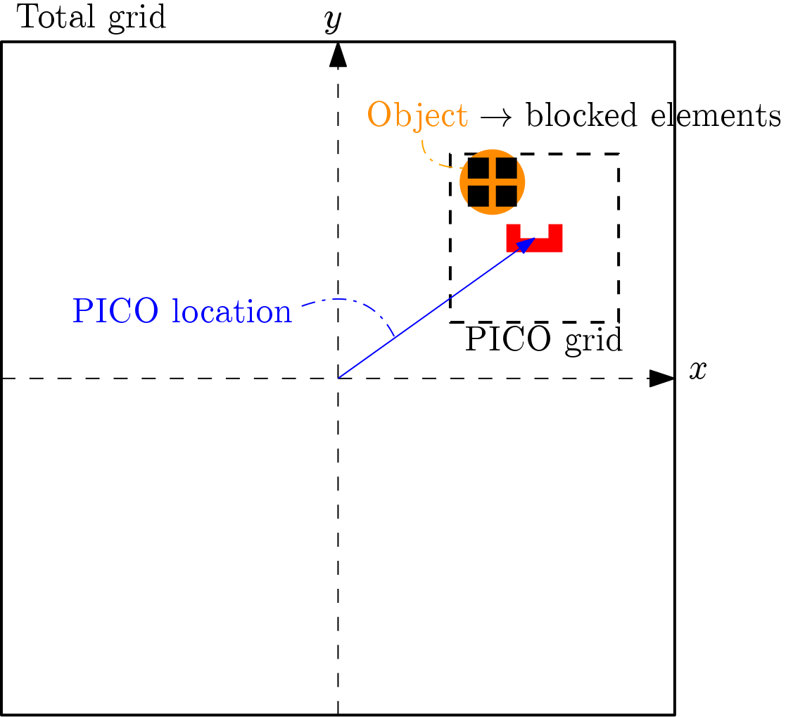
This object recognition does not have to be performed for the entire map during all the time steps. It can be done for all the map elements within a certain radius around PICO's current location on a low, for example, 1 Hz, frequency. To give a more specific example, a 4x4 [m] square around PICO's location is compared in the old and the new map. This is implemented by obtaining PICO's current location, also through a ROS callback, and drawing a grid of 4x4 [m] in elements around it. These elements are then compared between the current and the old map.

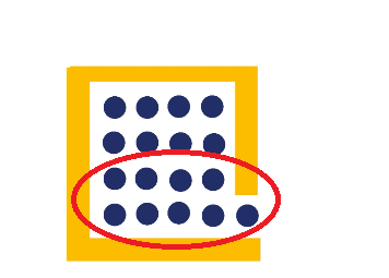
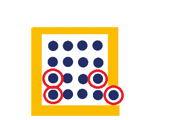
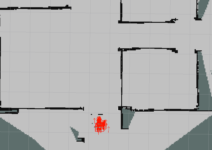
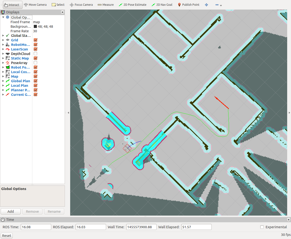
Since the current map size is 20x20 [m] with a resolution of 10 [cm] and it is assumed that the object is at least 20x20 [cm], an object is recognized if more than 4 elements are different in the old map compared to the live map. Note that this algorithm has not been implemented yet and could lead to problems if the live map changes parts of the map, with respect to the old map. If map parts that include walls are changed, either to blocked or non-blocked elements, the wall locations in the map could shift slightly. Since this would likely lead to differences in the old map compared to the live map this could be recognized as an object whereas it is just a slightly altered wall location. In order to prevent this, another ROS tool can be implemented to inflate the walls in the occupancy grid. This method is called costmap_2d [4], which "takes in sensor data from the world, builds a 2D or 3D occupancy grid of the data (depending on whether a voxel-based implementation is used), and inflates costs in a 2D cost map based on the occupancy grid and a user-specified inflation radius". In other words, it takes the occupancy grid data on the left figure below and transforms it into what is shown in the figure on the right below.

Hence, the area in which this algorithm searches for an object is within the 4x4 [m] square around PICO AND is in the non-blocked space of the cost map. This should, in theory, prevent the algorithm reacting to slight changes in the wall location (blocked space) in the occupancy grid. If an object is recognized for at least 10 samples to prevent any inaccuracies in the readings, a setpoint is set at the object's location and PICO moves towards it. After it reaches the object it stops and shouts "I found the object!".

As with most algorithms on this wiki, a visual representation makes the idea a lot clearer. The figure on the top-right shows a visual interpretation of PICO in the total grid (entire map) and a grid around PICO in which the algorithm compares maps to find the object. If an object is detected in the form of a number of newly detected blocked space elements within the cost map, PICO announces that it has found the object.

We did not manage to implement this part, unfortunately. However, it was discovered that if Gmapping is left running, it will not easily change non-blocked areas to blocked areas. Hence, objects are not always recognized completely. Since it has not been implemented, the method could not be tested and hence the severity of this problem could not be analyzed.

Figure X: Simple occupancy grid [1].

Figure X2: 2D costmap with inflation around objects/walls [2].

Executing the challenge

The execution of the challenge did go worse than planned. The wall follower did not work as smoothly as in the simulator, but in the end we were able to map the whole hospital floor. We were not successful in parking, because the robot was not back at its starting point before the challenge time ran out. A picture of the map that was created by PICO is shown below. Clicking on the picture will link to the youtube video of PICO performing the final challenge.

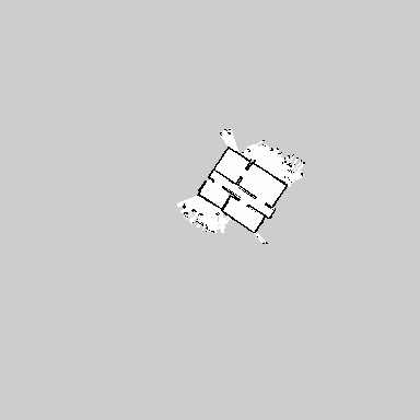
Even though we did not complete the full challenge, we managed to end in a third place!

We were still quite surprised by PICO's behaviour during the challenge, because in simulation it worked perfectly before (as can be seen in the part about the wall follower). Hence, we wanted to run a simulation with the final challenge's map to see if the behaviour is similar in this simulation map versus the actual hospital room. The simulation is found in this YouTube video of the simulation. (There were problems with uploading the GIF on the wiki).

While still not working perfectly, the simulation works a lot smoother than the actual challenge. As can be seen, it did sway from its path a number of times, but always found its way back in a decent manner using the incorporated fail-safes such as finding a wall (moving sideways to the right). Moreover, when the simulation returns to the start, it keeps turning. However, this would almost definitely not have happened in the challenge if it had returned to the start correctly, as the parking feature had been tested successfully a number of times before.

Note that during testing for the last time before the challenge, it did not run smoothly either. However, we could not get it fixed during the testing and every change we made after that could only be tested in simulation. Therefore, we knew beforehand that there was a good chance that PICO would not behave exactly as we wanted to since that was exactly the case before as well. If we would have had maybe one or two more hours to tune some parameters during testing, it could have potentially performed a lot better and in a similar manner to simulation.

Recommendations

• Try to get the basics of C++ down really well so that you know your way around the implementation

• In the first week we were told to focus on the initial design and really work out well what we, in theory, wanted to achieve. While this is a good idea, it can lead to wanting to have the best, smartest solution possible to solve the challenge. This happened to our group in a sense. We set out with great plans to create something beautiful, but after numerous setbacks, were not able to achieve this, making us have to re-think our plans nearly every week. I think the key idea to take from this is: start easy and improve. Of course, you could start taking bigger steps if you have more experience. However, seeing as we were all inexperienced in programming or doing something similar to this course, we should have started smaller, before thinking big.

• One of the key aspects of this project is separating the code into multiple smaller parts with clear in- and outputs. It is however very important to note that a general output like "an occupancy grid" might lead to problems. Each and every part has to be specified as far and as clearly as possible. To stick to the occupancy grid example this could, for example, be a double array with values -1, 0 and 100 with the value -1 zero unknown space, 0 free space and 100 occupied space. If the inputs are specified this clearly this leads to code that can be integrated relatively easy.

• Try to sit together with the group as often as possible. During these programming meetings, ideas can be discussed and problems can be solved much more easily than if people are working alone. The same holds for testing. If testing is done in a group this leads to much more knowledge in the group and problems can be solved much more easily.

• Write code part by part and test it as soon as possible, both in the simulator and in practice.

• Do not celebrate when the code works in simulation, because simulation is not the real world. Unfortunately, that was found the hard way.....

• Try to involve everybody in the project, because once you do not know what is going on in the code it is very hard to get into it.

• Have at least one specialist and one reviewer on each piece of code. This way there are always two people who know the code. These people can help each other if there are problems and this also means that it is not a dramatic problem if one of the team members is absent during for example testing.

• Think critically before you start coding. Do not start right away, but think about what input is needed, how this input can be used, what kind of output is desired and in what form this output can best be presented.

• Note that you do not have to reinvent the wheel all the time. If, due to for example a lack of time, it is not possible to write all the code from scratch know that there are a lot of libraries and packages that can help in reaching the desired goal. Note that these tools are not a holy grail and these tools should therefore only be used as a tool and not in any other way.

Code snippets

We based our code on three main goals:

- Efficiency

- Readability

- Testability

Efficiency

The bottleneck for most real-time controlling processes is the data flow. Due to that, we paid special attention to our data structure. Luckily C++ was designed especially for object-oriented programming, which made it easy to use its advantages during building an abstract structure. We tried to make the code as abstract as possible and group skills and tasks in functions and classes. In addition to that, we used pointers, which saves time and storage space during transfer processes. It makes a large difference if a complete class, function or list is passed around or just the location of the instance.

Readability

Indentations and free spaces make our code more readable. In addition to that comments are used to enable an easy and fast understanding. We used comments to explain more complicated processes and explain the functioning of each function. Nevertheless, we avoided over-commenting.

Due to the use of functions, classes, and blocks the code has a clear structure. For a better overview, classes are divided in header and .cpp files. Header files are only used for the definition of variables and functions. The actual code is found in the .cpp files. According to current coding standards we used in every class a constructor and destructor.

All object and variable names are based on their meaning. The naming is consistent for every code part.

Testability

Each program part provided a unit test. In this way, we were able to test each part separately during the development and localize errors more easily. We also could test unfinished code parts, that were not able to work in simulation or on the robot.

• Odom listener and TF broadcaster
• Potential field and first point detection
• Retrieve PICO location in map and the corresponding location header file