Embedded Motion Control 2013 Group 10: Difference between revisions
| Line 71: | Line 71: | ||
While performing these steps “wall-avoidance” keeps running. | While performing these steps “wall-avoidance” keeps running. | ||
In the next stadium of programming this node should become more robust and should constantly update and control the position. | In the next stadium of programming this node should become more robust and should constantly update and control the position. | ||
== Mapping == | |||
Revision as of 20:07, 29 September 2013
Group Name
Team Picobello
Group Members
| Name: | Student id: | Email: |
| Pepijn Smits | 0651350 | p.smits.1@student.tue.nl |
| Sanne Janssen | 0657513 | s.e.m.janssen@student.tue.nl |
| Rokus Ottervanger | 0650019 | r.a.ottervanger@student.tue.nl |
| Tim Korssen | 0649843 | t.korssen@student.tue.nl |
Positioning

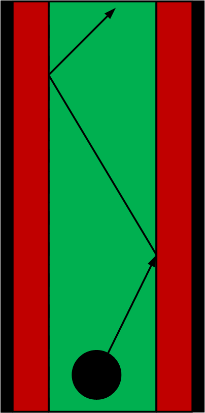
To remain in the center of the corridor and avoid hitting the wall the position is continuously checked and controlled. This is visualized in the picture below. The black area is the wall, the red area is close to the wall and should be avoided and the green area is the area where it is safe to drive. The robot drives forwards until it drives into the red area. Whether the robot is inside the red area is determined directly from the laserdata. If it is in the area it makes a slight turn (about 5 degrees) into direction of the green area and then again drives in forward direction.
Wall Avoidance

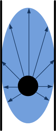
Wall avoidance has the highest priority at all times and is therefore active a all times. Wall avoidance measures distance in all possible directions. Once one distance becomes too small the “wall avoidance node” overrules all other nodes and commands the robot to stop. The threshold for the distance is not just a scalar. Since the robot has some velocity in forward direction, more space is required in forward direction of the robot than sideways. Therefore the threshold has an elliptic profile as shown in the figure.
Noise reduction
To reduce noise a Gaussian filter is added. [math]\displaystyle{ G(x)=\frac{1}{\sqrt{2 \pi}}e^{\frac{-x^2}{2 \sigma^2}} }[/math]
This Gaussian function is used to make a 9x1 Kernel. So that every point is the weighted averaged of 9 measurements. This results in the following kernel for [math]\displaystyle{ \sigma=2 }[/math]:
g = [0.0276 0.0663 0.1238 0.1802 0.2042 0.1802 0.1238 0.0663 0.0276]
So that the sum(g) = 1.
Corner detection
If there is a corner there is a sudden bump in the obtained laserdata. The location of this bump can be determined with the gradient of the laserdata. Since we still want to filter the data a kernel is used based upon the gradient of the Gaussian. [math]\displaystyle{ \nabla G(x)=\frac{-x}{\sigma^2}\frac{1}{\sqrt{2 \pi}}e^{\frac{-x^2}{2 \sigma^2}} }[/math]
Resulting in the following kernel for [math]\displaystyle{ \sigma=2 }[/math]:
dg=[0.1353 0.2435 0.3033 0.2206 0 -0.2206 -0.3033 -0.2435 -0.1353]
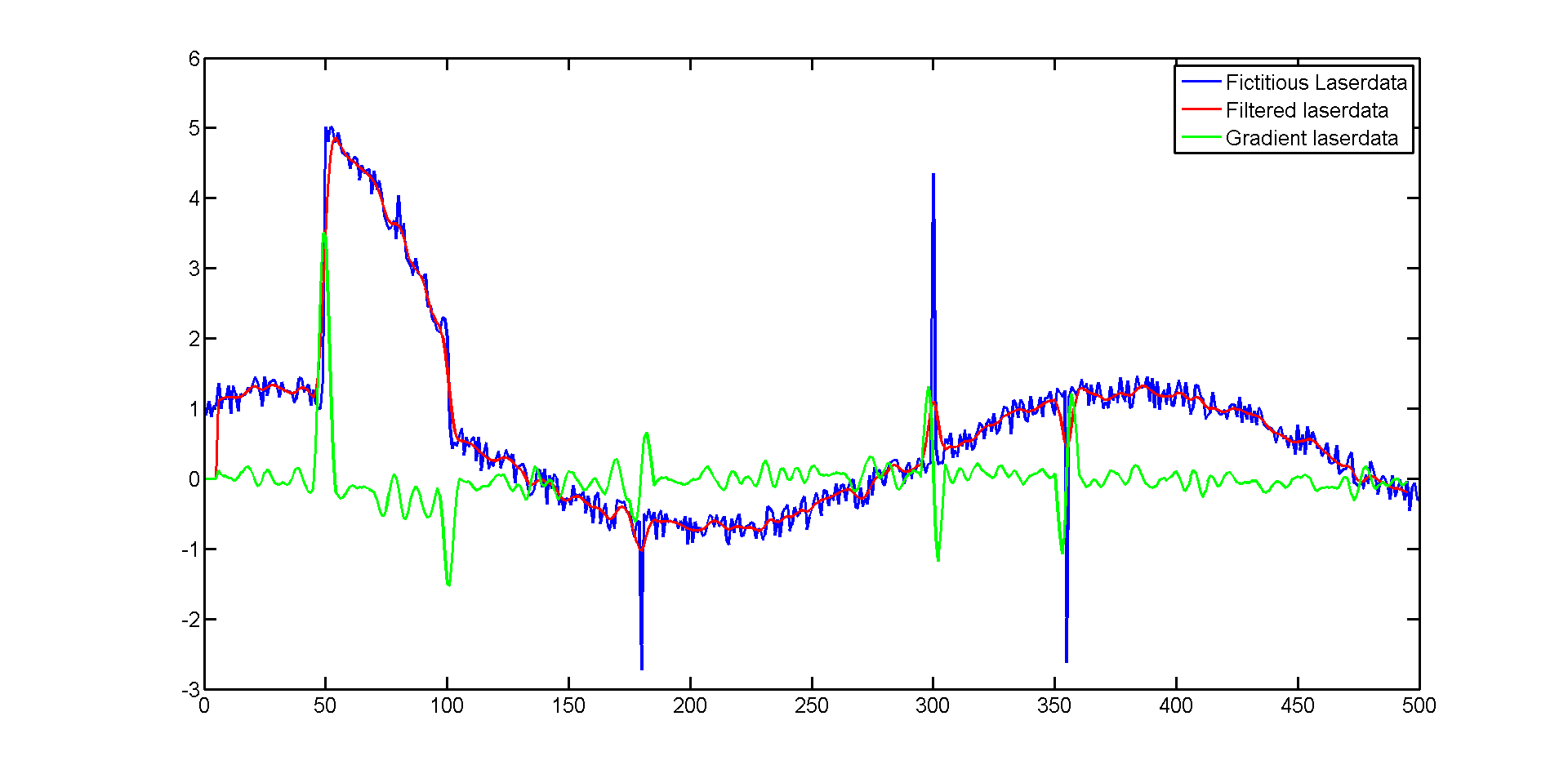
The way corners are detected can be visualized using some fictitious laserdata. We see some laserdata with both white noise as well as salt and pepper noise. The Gaussian filters the noise reasonably. The size of the kernel should be tuned. A larger kernel results in less noise, but results in more loss of data. The green line shows the gradient of the laser data. If a proper threshold is chosen this can be used to determine a bump in distance and thus a corner.

Corner movement

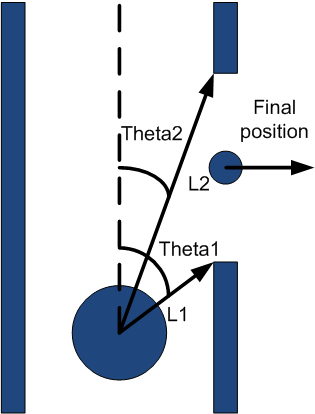
If there is a sideway, two corners are detected. The distance and corresponding angle towards each of those corners are sent towards the “go-around-corner-node”. Once theta1 is about + or – 90 degrees this nodes takes the following steps:
- Drive forward until L1=L2
- Turn towards corner until theta1 = theta 2
- Drive forward until theta1 > 90 degrees and theta2 < 90 degrees.
While performing these steps “wall-avoidance” keeps running. In the next stadium of programming this node should become more robust and should constantly update and control the position.