Integration Project Systems and Control 2013 Group 2

Group Members

Name:	Student id:	Email:
Rens Samplonius	0785119	r.j.samplonius@student.tue.nl
Frank Evers	0789890	f.evers@student.tue.nl
Juan Guo	0825223	j.guo@student.tue.nl
Jeroen Lamers	0771264	j.w.lamers@student.tue.nl

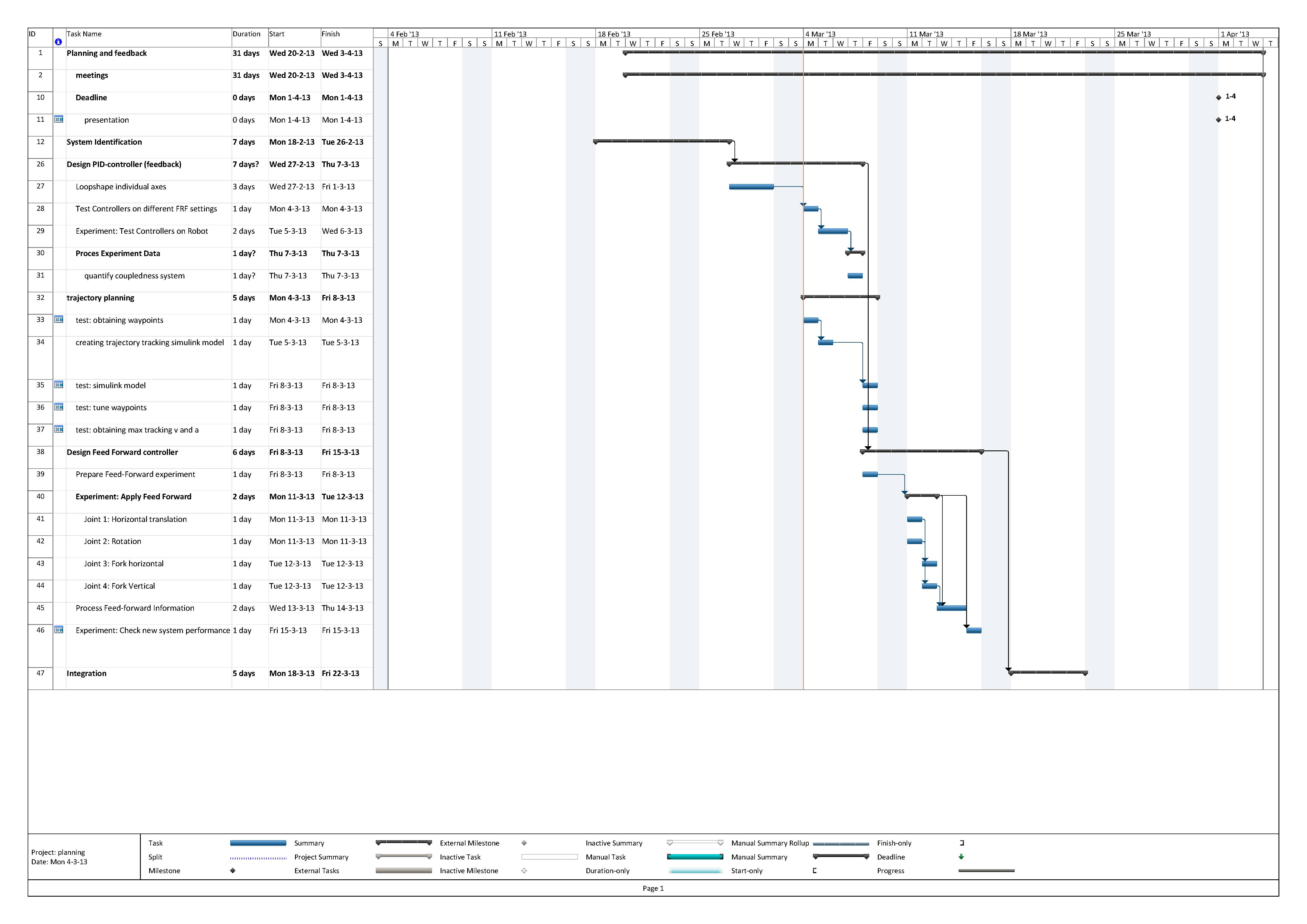
Planning

Week 1

- Project planning

- Familiarization with the robot

- Literature searching

- Define specifications of the control system

( This will be the guide for the control system design. As a complete list of requirements can help insure the overall performance and stability of the system. This can avoid the redesign of the controller, when certain important specifications are found to be not satisfied afterwards.One problem of having a complete list of requirements is the trade-off among them, which has to be evaluated based on the importance of the requirement.)

Week 2

- FRF measurement

( Modeling of the system is the first step to its control algorithm design. Two main modeling method we know: physical modeling and data based modeling. Physical modeling is based on conservation law. The system we face is pretty complex and certain phisical phenomina which can have a big influence on the dynamics of the system such as friction is hard to model in this way; also parameters like mass and inertia are not provided directly. Thus we choose data based modeling. Both frequency response measurements (linear system) and system identification method will be used.)

Week 3

- PID controller design and its discretization

(PID controller for sure will control the system to a degree. Start from this simply but powerful controller we can have some idea of control effort required to achieve a good performance of the system. Later modification and alternative control algorithms will be considered if the performance is not satisfying. Controller discretization will be considered if the discrete model in Simulink works poorly.)

Week 4

- PID controller combined with feedforward controller design

( To achieve a good trajectory tracking only the PID controller is not enough. As it only react to existing error signal. Adding feedforward controller to correct error beforehand will improve trajectory tracking. )

Week 5

- Trajectory planning and controller testing

- Modeling by system identification

Progress

Week 1

1) Literature collecting and background knowledge review.

2) Control system requirement design:

 <1>  All pizzas have to be moved from left to right under 15 seconds.
 <2>  Reference profile has to optimal in the sense of output [V]. (frank what do u mean by this???)
 <3>  During transport the pizza should remain on the robot. 
 <4>  Controllers design: stability and performance requirement.
     <*>  Frequency domain
         - Bandwidth for complementary sensitivity of individual axis aim for relatively large bandwidth.
         - Big cut-off rate the slop of magnitude plot at high frequency of individual axis.
         - Resonance peak between 1dB to 1.5dB for individual axis.
         - For open loop, generally we require low frequency high gain and high frequency low gain.
         - For sensitivity, we require low frequency low gain.
         - Relatively big gain margin and phase margin.
     <*>  Time domain
         - Step or impulse response performance (open loop response), i.e. rise time, overshoot, settling time, steady state error bound.
         - Required tracking error individual controller. (Vertical fork x = mm; Horizontal fork y = ..mm; Rotation θ = ..mm; Table translation z = ..mm.)
 <5>  The complete trajectory has to be splitted in sub trajectories, which have to be executed in the required times. (frank maybe u modify this later.)
 <6>  Boundary conditions for actuators. (can anyone fill this up? thx)

3) Familiarization of the robot. | - Initialization 4 axis

Week 2

• Rens and Jeroen conducted an FRF measurement on the left pizza robot. They did a closed loop measurement on each axis by applying a sin-wave + white noise to the plant. The sine wave is added to overcome the massive friction. The controller used in the closed loop measurement is tuned very low. During the FRF measurement the following data is collected: the input signal (u), the white noise signal (w), and the output voltages (v). With this data we calculated the process sensitivity and the sensitivity and to obtain the plant we divided them (similar as we did during the Motion Control course). We are uncertain if the left and right pizza robots have a similar plant so perhaps we should repeat the FRF measurement on the right robot because that one has the pizza racks on it.

Week 3

• We decided to use PID controller to control the pizza robot because we all have the most experience with them. This week we evaluated the FRF measurement data and loaded this in the programme ShapeIt. Because the right pizza robot broke we were not able to do more because we scheduled testing time on that robot.

Week 4

• We designed four controllers for each axis with a bandwidth of approx. 10Hz. We also obtaind all the positions to pickup the pizzas. With these positions we start to constuct the optimal trajectory.