Embedded Motion Control 2016 Group 4: Difference between revisions
| Line 184: | Line 184: | ||
=== '''Laser Range Finder''' === | === '''Laser Range Finder''' === | ||
<ul> | |||
<li><p>Observation relative to robot <math>z = h(x_v,x_f,w)</math></p> | |||
{| | |||
| <math> x_v </math>: | |||
| robot state | |||
|- | |||
| <math> x_f </math>: | |||
| location of feature | |||
|- | |||
| <math> w </math>: | |||
| sensor error | |||
|} | |||
</li> | |||
<li><p>Observation of feature <math> i </math> <math>z = | |||
\begin{bmatrix} | |||
r\\\beta | |||
\end{bmatrix} | |||
= | |||
\begin{bmatrix} | |||
\sqrt{(y_i - y_v)^2 + (x_i - x_v)^2}\\ | |||
\tan{^{-1} }\frac{y_i-y_v}{x_i - x_v} - \theta_v | |||
\end{bmatrix} | |||
+ | |||
\begin{bmatrix} | |||
w_r\\w_\beta | |||
\end{bmatrix}</math></p> | |||
{| | |||
| <math> r </math>: | |||
| range | |||
|- | |||
| <math> \beta </math>: | |||
| bearing angle | |||
|} | |||
</li> | |||
<li><p>Linearize equation</p></li></ul> | |||
=== '''Extended Kalman Filter''' === | === '''Extended Kalman Filter''' === | ||
Revision as of 03:00, 15 June 2016
Group Members
| ID-Number | Name | |
| 0811028 | Tim Josten | t.j.josten@student.tue.nl |
| 0790737 | Tom Leenen | t.c.p.f.leenen@student.tue.nl |
| 0832751 | Martin Plantinga | m.plantinga@student.tue.nl |
| 0816951 | Joey Reinders | j.m.f.reinders@student.tue.nl |
Goal
The goal of this project is to make a robot (PICO or TACO) navigate autonomously and as seamlessly as possible through a maze and find the exit. The robot has a computer integrated in it that runs on Linux, with ROS (Robot Operating System) running on top. The software has to be written in the C++ programming language. To achieve the goal, a software architecture has to be designed that structurally makes room for the different requirements, functions, components, specifications and interfaces.
Requirements
To achieve the final goal several requirements are determined, which can be seen in the following list.
- Navigate autonomously to the exit of the maze as fast as possible
- cruise as fast as possible while maintaining the different abilities
- Navigate autonomously to the exit of the maze as fast as possible
- Avoid obstacles
- recognize the different obstacles (e.g. walls) and keep a "safe" distance from them
- Avoid obstacles
- Avoid getting trapped in a loop of the maze
- recognize if the robot is navigating through the same path over and over and exit the loop
- Avoid getting trapped in a loop of the maze
- Create a map of the maze
- Recognize door, open it and drive through it
- Navigate in open spaces
- navigate if no obstacle is in sight
- Navigate in open spaces
- Scalable system
- the software should be able to work independently of the size and structure of the maze
- Scalable system
Functions
The functions can be divided into two groups: the basic functions and the skill functions. The basic functions are basic actions that the robot will do. The skill functions are a set of actions to accomplish a certain goal.
The basic functions consist of:
- Actuation of the robot:
- Provide signals to the actuators of the robot. Realize the desired motion by using a controller and meeting the requirements.
- Input: location of robot, Output: motion of robot
- Actuation of the robot:
- Detect:
- Characterize different types of corridors based on telemetry provided by the Laser Range Finder (LRF).
- Input: measured x, y and theta; Output: type of corridor
- Detect:
The skill functions consist of:
- Mapping:
- Create and update a map of the explored maze. The robot will recall this map as its future moves will depend on this map.
- Input: current x, y and theta of the robot; Output: new/updated maze map, new/adjusted objective of the robot.
- Mapping:
- Feedback:
- Check position of robot with position of the created map. Prevent the robot from collisions with the walls or other obstacles.
- Input: current x, y, theta, LFR data and objective; Output: motion of the robot.
- Feedback:
- Decision:
- Check position of robot with position of the created map. Prevent the robot from collisions with the walls or other obstacles.
- Input: current x, y, theta, LFR data and objective; Output: motion of the robot
- Decision:
- Monitor:
- Control the exploration of the maze and prevent the robot from getting stuck in a loop.
- Input: current x, y and theta of the robot; Output: previously unexplored area
- Monitor:
- Door check:
- Wait at the potential door location for a predetermined time period while scanning the distance to the potential door to check if it opens.
- Input: current x, y and theta of the robot; Output: A door that either opens or stays closed, followed by pico's new objective based upon the result.
- Door check:
- Obstacle check:
- Measure the preset minimum safe distance from the walls or measure not moving as expected according to the driving action.
- Input: current and expected x, y and theta of the robot; Output: new motion of the robot based upon the result.
- Obstacle check:
Components
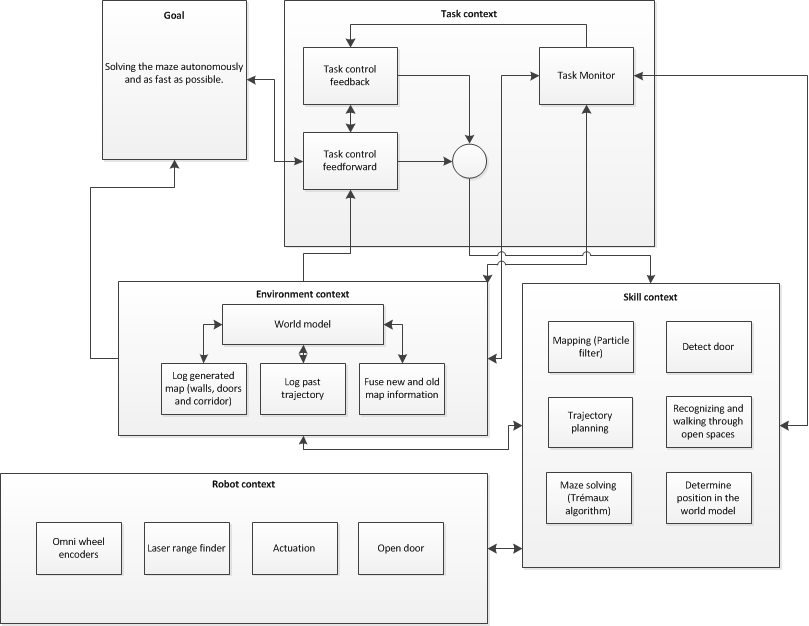
To fulfilll the previously mentioned functions and achieve the goal, the software should contain different components that interact with each other. This can be seen in Figure 1.
The C++ code should contain the components shown in Figure 1. There should be a task manager to switch between different tasks. An algorithm should be made that decides which task is performed or whether different tasks are performed simultaneously.
An algorithm should be implemented for controlling the robot and accurately position it, this algorithm uses the environment model, which is made using the laser range finder and omni-wheel encoders. This world model is logged and will be continuously updated during the maze solving of the robot.
The robot should have several skills and these should be programmed effectively with a fast algorithm. For the world model, the robot needs a mapping skill and it needs to determine its position in this world model. To solve the maze the robot needs a trajectory planning which uses an effcient maze solving algorithm (e.g. Trémaux).
Eventually when the robot has solved the maze, the algorithm has to be stopped.

Specifications
In the specifications the tasks that the robot has to conduct are quantified (i.e. given a value).
- The maximal translational velocity of PICO is 0.5 m/s
- The maximal rotational speed of PICO is 1.2 rad/s
- PICO has to solve the corridor challenge within 5 minutes
- PICO has to solve the maze challenge within 7 minutes
- PICO may not stop moving for more than 30 seconds (e.g. when opening the door)
Interfaces
To interpret the data that the robot collects, it is convenient to make a graphical user interface that visualizes this data. The omni-wheel encoder in combination with the laser range finder can be used to visualize the path of the robot and make the world model. The encoder data should be transformed to robot coordinates with a kinematic model of the robot.
The laser range finder also produces data, and to see if this data is interpreted in the right way a visualization should be made. It can be used to see if walls, doors and exits are detected in the right way. Possible algorithms for this are the Hough transform and particle filter.
Software architecture & approach
In Figure 2 the software architecture can be seen. Two sensors are being used: the laser range finder, which is used to generate a potential field and to discover features and the encoder data, which is used to generate a map of the maze. The detected features form the map together with the encoder data. A target will be picked based upon this map to set a target. The potential field will help Pico with reaching this target. This potential field will let Pico drive in the direction where it should go.

Methods
Node detection
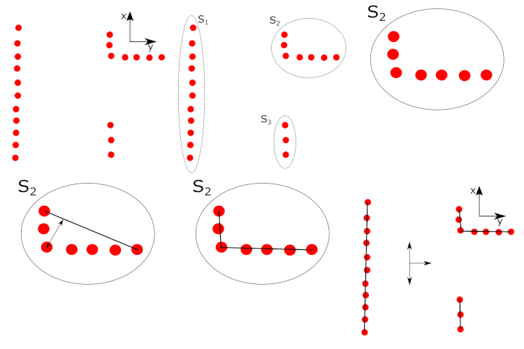
The node detection is done by using line extraction (Split and Merge). This is done as follows:
- Compute local x and y coordinates based on LRF
- Compute sets of data based on distance between points
- Fit straight lines through separate sets
- Determine maximal error and split set again
- Repeat 3 and 4 until maximal error is small enough
- Determine nodes local position and type
The node detection algorithm is visually shown in Figure 3.

Position estimation
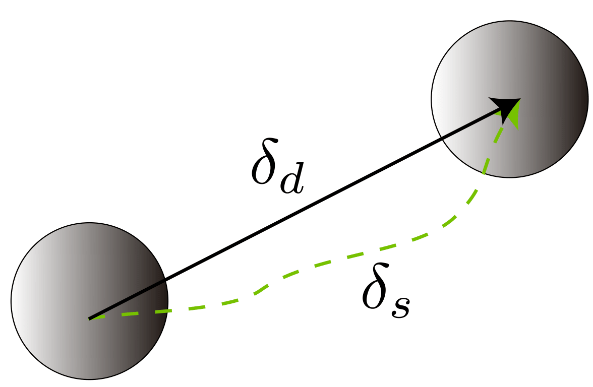
To estimate the position of Pico, odometry data is used. And since the frequency is high, the motions are relatively small and it is assumed that: [math]\displaystyle{ \delta_d= \delta_s }[/math] which can be seen in Figure 4.

SLAM
Equations of Motion
Discrete-time model [math]\displaystyle{ x_{{\langle k+1 \rangle}}= f(x_{{\langle k \rangle}}, \delta_{{\langle k \rangle}}, v_{ {\langle k \rangle}}) }[/math]
New configuration in terms of previous configuration and odometry
[math]\displaystyle{ \xi_{{\langle k+1 \rangle}}= \begin{bmatrix} x_{{\langle k \rangle}}+ (\delta_{d,{{\langle k \rangle}}}+v_d)\cos(\theta_{{\langle k \rangle}}+\delta_\theta + v_\theta)\\ y_{{\langle k \rangle}}+ (\delta_{d,{{\langle k \rangle}}}+v_d)\sin(\theta_{{\langle k \rangle}}+\delta_\theta + v_\theta)\\ \theta_{{\langle k \rangle}}+ \delta_\theta + v_\theta \end{bmatrix} }[/math][math]\displaystyle{ \delta_d }[/math]: movement in x direction [math]\displaystyle{ \delta_\theta }[/math]: rotation [math]\displaystyle{ v_d, v_\theta }[/math]: error in odometry
Laser Range Finder
Observation relative to robot [math]\displaystyle{ z = h(x_v,x_f,w) }[/math]
[math]\displaystyle{ x_v }[/math]: robot state [math]\displaystyle{ x_f }[/math]: location of feature [math]\displaystyle{ w }[/math]: sensor error Observation of feature [math]\displaystyle{ i }[/math] [math]\displaystyle{ z = \begin{bmatrix} r\\\beta \end{bmatrix} = \begin{bmatrix} \sqrt{(y_i - y_v)^2 + (x_i - x_v)^2}\\ \tan{^{-1} }\frac{y_i-y_v}{x_i - x_v} - \theta_v \end{bmatrix} + \begin{bmatrix} w_r\\w_\beta \end{bmatrix} }[/math]
[math]\displaystyle{ r }[/math]: range [math]\displaystyle{ \beta }[/math]: bearing angle Linearize equation
Extended Kalman Filter
Map Making
Simultaneous Localization and Mapping
Path planning
Difficult Problems
Content
Corridor Challenge
Content
Maze Challenge
Content
Documents
- Initial design document (week 1): File:InitialDesignIdea - Group 4.pdf
- Design presentation (week 4): File:Design Presentation.pdf
- Final presentation (week 8): File:Final Presentation.pdf