Embedded Motion Control 2015 Group 3: Difference between revisions
| Line 198: | Line 198: | ||
= Localisation = | |||
The localisation algorithm is explained in the section below, by separating and discussing the important factors. | The localisation algorithm is explained in the section below, by separating and discussing the important factors. | ||
== Purpose of Localisation == | |||
The purpose of the localisation is that the robot can prevent itself from driving in a loop for infinite time, by knowing where it is at a given moment in time. By knowing where it is, it can decide based on this information what to do next. As a result, the robot will be able to exit the maze within finite time, or it will tell there is no exit if it has searched everywhere without success. | The purpose of the localisation is that the robot can prevent itself from driving in a loop for infinite time, by knowing where it is at a given moment in time. By knowing where it is, it can decide based on this information what to do next. As a result, the robot will be able to exit the maze within finite time, or it will tell there is no exit if it has searched everywhere without success. | ||
== Requirements of Localisation == | |||
In order to be able to locate itself within its environment, the robot needs information. The is required to obtain global position data: | In order to be able to locate itself within its environment, the robot needs information. The is required to obtain global position data: | ||
| Line 220: | Line 220: | ||
# velocity input to robot | # velocity input to robot | ||
== Method of localisation == | |||
The robot will need global coordinates. There are two sensors which it can use to determine these coordinates. However both sensors have their own drawbacks. | The robot will need global coordinates. There are two sensors which it can use to determine these coordinates. However both sensors have their own drawbacks. | ||
*The odometry sensor provides global x-y coordinates and angle. There is not much variance in the data of the sensor, but there is a drift (bias) that will accumulate over time. The odometry data can be viewed as feedforward information for the system. | *The odometry sensor provides global x-y coordinates and angle. There is not much variance in the data of the sensor, but there is a drift (bias) that will accumulate over time. The odometry data can be viewed as feedforward information for the system. | ||
| Line 230: | Line 230: | ||
A '''Kalman filter''' is used to filter the data obtained from odometry as well as from LRF, in order to maximize the accuracy. | A '''Kalman filter''' is used to filter the data obtained from odometry as well as from LRF, in order to maximize the accuracy. | ||
=== Kalman filter === | |||
The kalman filter uses an update cycle with two steps. In the first step the new position is estimated based on the previous position and the input. An estimate of its error is then made which is used in the second step. In the second step data from measurements is used to correct the estimated position. Since the definition of the directions of the x and y axis is arbitrary, they are aligned to the corridor in which pico starts. The algorithm that is used is shown in the figure below: | The kalman filter uses an update cycle with two steps. In the first step the new position is estimated based on the previous position and the input. An estimate of its error is then made which is used in the second step. In the second step data from measurements is used to correct the estimated position. Since the definition of the directions of the x and y axis is arbitrary, they are aligned to the corridor in which pico starts. The algorithm that is used is shown in the figure below: | ||
| Line 274: | Line 273: | ||
Since it is possible to lose sight of a wall, for instance when driving on an intersection, a safeguard is put in place. If the position change based on the lrf is to big, it is assumed that the LRF data is unreliable for that update cycle and only the odometry data is used. This is done by switching between two R matrices, one of which sets the contributions of the laserdata to zero. In the regular R matrix the contribution of the LRF data is weighed more heavily under the assumption that the LRF is more reliable overall. | Since it is possible to lose sight of a wall, for instance when driving on an intersection, a safeguard is put in place. If the position change based on the lrf is to big, it is assumed that the LRF data is unreliable for that update cycle and only the odometry data is used. This is done by switching between two R matrices, one of which sets the contributions of the laserdata to zero. In the regular R matrix the contribution of the LRF data is weighed more heavily under the assumption that the LRF is more reliable overall. | ||
== Implementation of method == | |||
===Interface=== | |||
==== Retreiving Velocity data ==== | |||
==== Retreiving Odometry data ==== | |||
==== Retreiving LRF data ==== | |||
=== Initializing position === | |||
=== Calculating coordinates from LRF === | |||
=== Implementation of Kalman filter === | |||
== Technicalities == | |||
Revision as of 11:42, 9 June 2015
This is the Wiki-page for EMC-group 3.
Group members
| Name | Student number | |
|---|---|---|
| Max van Lith | 0767328 | m.m.g.v.lith@student.tue.nl |
| Shengling Shi | 0925030 | s.shi@student.tue.nl |
| Michèl Lammers | 0824359 | m.r.lammers@student.tue.nl |
| Jasper Verhoeven | 0780966 | j.w.h.verhoeven@student.tue.nl |
| Ricardo Shousha | 0772504 | r.shousha@student.tue.nl |
| Sjors Kamps | 0793442 | j.w.m.kamps@student.tue.nl |
| Stephan van Nispen | 0764290 | s.h.m.v.nispen@student.tue.nl |
| Luuk Zwaans | 0743596 | l.w.a.zwaans@student.tue.nl |
| Sander Hermanussen | 0774293 | s.j.hermanussen@student.tue.nl |
| Bart van Dongen | 0777752 | b.c.h.v.dongen@student.tue.nl |
General information
This course is about software design and how to apply this in the context of autonomous robots. The accompanying assignment is about applying this knowledge to a real-life robotics task.
The goal of this course is to acquire knowledge and insight about the design and implementation of embedded motion systems. Furthermore, the purpose is to develop insight in the possibilities and limitations in relation with the embedded environment (actuators, sensors, processors, RTOS). To make this operational and to practically implement an embedded control system for an autonomous robot in the Maze Challenge, in which the robot has to find its way out in a maze.
PICO is the name of the robot that will be used. Basically, PICO has two types of inputs:
- The laser data from the laser range finder
- The odometry data from the wheels
In the fourth week there is the "Corridor Competition". During this challenge, called the corridor competition the students have to let the robot drive through a corridor and then take the first exit.
At the end of the project, the "A-maze-ing challenge" has to be solved. The goal of this competition is to let PICO autonomously drive through a maze and find the exit.
Design
In this section the general design of the project is discussed.
Requirements
The final goal of the project is to solve a random maze, fully autonomously. Based on the description of the maze challenge, several requirements can be set:
- Move and reach the exit of the maze.
- The robot should avoid bumping into the walls.
- So, it should perceive its surroundings.
- The robot has to solve the maze in a 'smart' way.
Functions & Communication
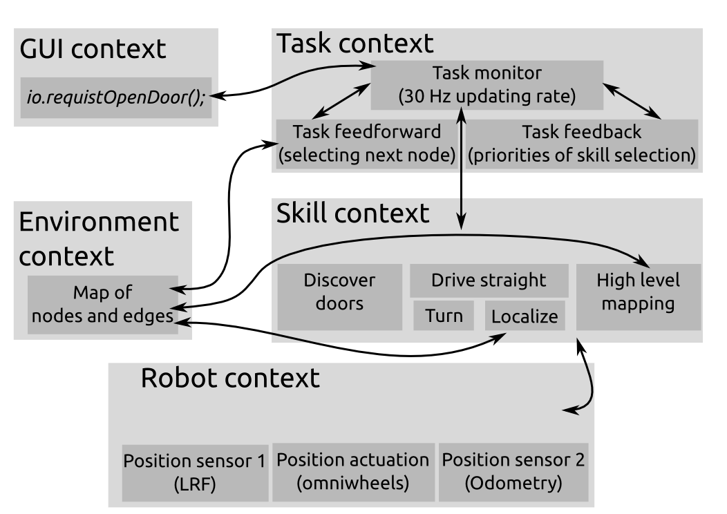
The robot will know a number of basic functions. These functions can be divided into two categories: tasks and skills.
The task are the most high level proceedings the robot should be able to do. These are:
- Determine situation
- Decision making
- Skill selection
The skills are specific actions that accomplish a certain goal. The list of skills is as follows:
- Drive
- Rotate
- Scan environment
- Handle intersections
- Handle dead ends
- Discover doors
- Mapping environment
- Make decisions based on the map
- Detect the end of the maze
Structure
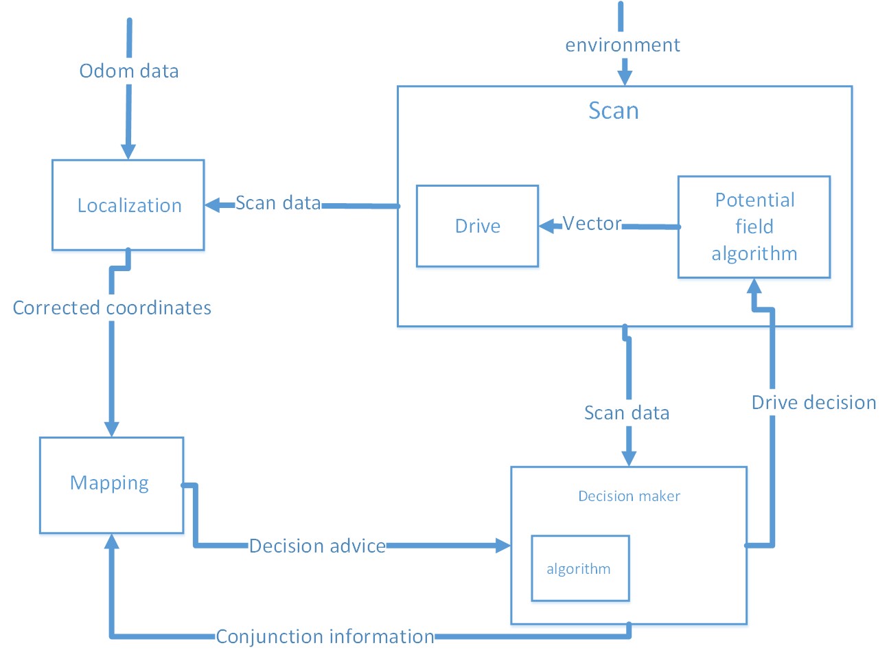
The problem is divided into different blocks. We have chosen to make these four blocks: Drive, Scan, Decision and Mapping. The following is an overall structure of the software:
Calibration
Calibration part (if we want)
...
...
Software implementation
In this section, implementation of this software will be discussed based on the block division we made.
Brief instruction about one block can be found here. In addition, there are also more detailed problem-solving processes and ideas which can be found in the sub-pages of each block.
Drive block
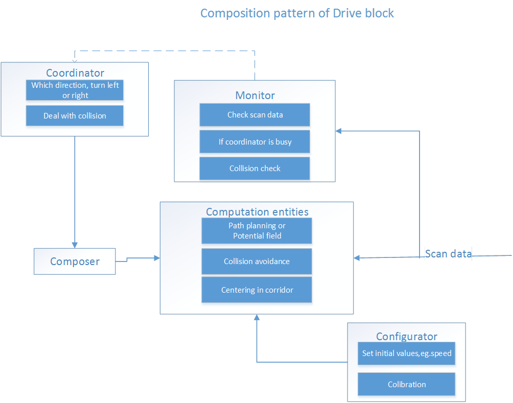
Basically, this block is the doer (not the thinker) of the complete system. In our case, the robot moves around using potential field. How the potential field works in detail is shown in Scan. Potential field is an easy way to drive through corridors, and making turns.
Two other methods were also considered: Simple method and Path planning. However, the potential field was the most robust and easiest method.
The composition pattern of the drive block:
Scan block
The block Scan processes the laser data of the Laser Range Finders. This data is used to detect corridors, doors and different kind of junctions. The data that is retrieved by 'scan' is used by all three other blocks.
- Scan directly gives information to 'drive'. Drive uses this to avoid collisions.
- The scan sends its data to 'decision' to determine an action at a junction for the 'drive' block.
- Mapping also uses data from scan to map the maze.
Potential field
By splitting up the received laser data from the LRF in x and y, and summing them up results in a large vector containing the appropiate angle for PICO to follow. In other words, PICO moves always to the place with the most space. Note, the actual magnitude of this resultant vector is of no importance, since the Drive block has is own conditions for setting the velocity.
In straight corridors PICO will drive in the middle in a robust manner with the help of the potential field. In the case that PICO approaches a T-junction or intersection a decision must be made by the decision maker.
Constructing virtual walls
At junctions and intersections the current potential field is unable to lead PICO to the desired direction. Therefore, an extra layer is added to the scan data which enables editing of the LRF data that pico will see. The main advantage of introducing this second layer is that the actual measured data still is availble for all different kind of processes used at different blocks. By modifying the data virtual walls are constructed, this will steer pico into the desired direction by using the potential field. The 'decision maker' in combination with the 'mapping algorithm' will decide were to place the virtual walls.
Collision avoidance
To create an extra layer of saftey avoidance collision has been added on top of the potential field. In general the potential field avoids collisions, however when constructing virtual walls fails the robot may crash into a wall and the turn of solving the maze is over. This avoidance collision is fairly easy, when the distance of multiple oextensive LRF beams is below a certain value PICO will move in the opposite direction. The usage of multiple beams is used to make this method more robust. The current parameter for activating avoidance collision is set at 30 centimeters measured from the its scanner, note that this valued is based on the dimensions of PICO.
Decision block
The decision block contains the algorithm for solving the maze. It can be seen as the 'brain' of the robot. It receives the data of the world from 'Scan'; then decides what to do (it can consult 'Mapping'); finally it sends commands to 'Drive'.
Input:
- Mapping model
- Scan data
Output:
- Specific drive action command
The used maze solving algorithm is called: Trémaux's algorithm. This algorithm requires drawing lines on the floor. Every time a direction is chosen it is marked bij drawing a line on the floor (from junction to junction). Choose everytime the direction with the fewest marks. If two direction are visited as often, then choose random between these two. Finally, the exit of the maze will be reached. (ref)
Different situations when visiting a node
* If it is a dead-end node
* Did the door open for me
* Any unvisited paths
* Any paths with 1 visit
* Paths with 2 visit (not a choice)
Mapping block
This block will store the corridors and junctions of the maze. Therefore, the decision block can consider certain possiblilities, to ensure that the maze will be solved in a strategic way.
As is said in the previous paragraph, the Tremaux algorithm is used: [1].
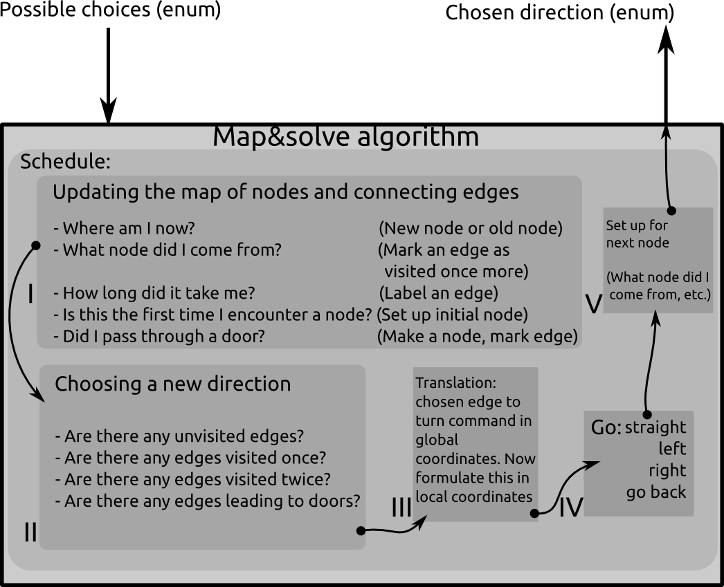
The maze will consist of nodes and edges. A node is either a dead end, or any place in the maze where the robot can go in more than one direction. an edge is the connection between one node and another. An edge may also lead to the same node. In the latter case, this edge is a loop. The algorithm is called by the general decision maker whenever the robot encounters a node (junction or a dead end). The input of the algorithm is the possible routes the robot can go (left, straight ahead, right, turn around) and the output is a choice of possible directions that will lead to solving the maze.
The schedule looks like this:
- Updating the map:
- Robot tries to find where he is located in global coordinates. Now it can decide if it is on a new node or on an old node.
- The robot figures out from which node it came from. Now it can define what edge it has been traversing. It marks the edge as 'visited once more'.
- All sorts of other properties may be associated with the edge. Energy consumption, traveling time, shape of the edge... This is not necessary for the algorithm, but it may help formulating more advanced weighting functions for optimizations.
- The robot will also have to realize if the current node is connected to a dead end. In that case, it will request the possible door to open.
- Choosing a new direction:
- Check if the door opened for me. In that case: Go straight ahead and mark the edge that lead up to the door as Visited 2 times. If not, choose the edge where you came from
- Are there any unvisited edges connected to the current node? In that case, follow the edge straight in front of you if that one is unvisited. Otherwise, follow the unvisited edge that is on your left. Otherwise, follow the unvisited edge on your right.
- Are there any edges visited once? Do not go there if there are any unvisited edges. If there are only edges that are visited once, follow the one straight ahead. Otherwise left, otherwise right.
- Are there any edges visited twice? Do not go there. According to the Tremaux algorithm, there must be an edge left to explore (visited once or not yet), or you are back at the starting point and the maze has no solution.
- Translation from chosen edge to turn command:
- The nodes are stored in a global coordinate system. The edges have a vector pointing from the node to the direction of the edge in global coordinates. The robot must receive a command that will guide it through the maze in local coordinates.
- The actual command is formulated
- A set-up is made for the next node
- e.g., the current node is saved as a 'nodeWhereICameFrom', so the next time the algorithm is called, it knows where it came from and start figuring out the next step.
Localisation
The localisation algorithm is explained in the section below, by separating and discussing the important factors.
Purpose of Localisation
The purpose of the localisation is that the robot can prevent itself from driving in a loop for infinite time, by knowing where it is at a given moment in time. By knowing where it is, it can decide based on this information what to do next. As a result, the robot will be able to exit the maze within finite time, or it will tell there is no exit if it has searched everywhere without success.
Requirements of Localisation
In order to be able to locate itself within its environment, the robot needs information. The is required to obtain global position data:
- global x-position [m]
- global y-position [m]
- global a-angle [rad.]
The error in the position data must be quantified and must be minimized, in order not to make mistakes in the location in the long run. For example, if the robots x-and y-coordinates differ due to an error, the robot will think is it at a different location, whereas it actually is standing still in exactly the same location and position.
The sensor data required to obtain the above mentioned position data are the following:
- odometry: global x [m] , global y [m] , global a [rad.]
- LRF: all laser ranges [m]
- velocity input to robot
Method of localisation
The robot will need global coordinates. There are two sensors which it can use to determine these coordinates. However both sensors have their own drawbacks.
- The odometry sensor provides global x-y coordinates and angle. There is not much variance in the data of the sensor, but there is a drift (bias) that will accumulate over time. The odometry data can be viewed as feedforward information for the system.
- The LRF sensor provides 1000 ranges [m] with distances to objects over a scope of 270 degreess around the robot. This sensor shows no bias, but has a variance however. Furthermore the LRF data does not provide the global coordinates that we want with its raw data. Therefore these ranges data have to be converted into additions to the global coordinates. The LRF data can be seen as the Feedback loop of the system.
When the robot starts its program initially, the global coordinates will be all zero. So the start position of the robot determines the direction of the x- and y-axes. The data from the odometry and the LRF will be updated at each time instant. The odometry just works very intuitively: it tells you how far you have moved based on wheel-rotation. In the case of LRF however, the following happens: It measures the distances to the objects in the environment at time t0. It measures again at t1. The difference in distance, converted to the wanted coordinates, should be equal to the odometry data. Of course this will not happen due to the errors in the sensors, but that is why a filter is used to filter the data in between each next update step.
A Kalman filter is used to filter the data obtained from odometry as well as from LRF, in order to maximize the accuracy.
Kalman filter
The kalman filter uses an update cycle with two steps. In the first step the new position is estimated based on the previous position and the input. An estimate of its error is then made which is used in the second step. In the second step data from measurements is used to correct the estimated position. Since the definition of the directions of the x and y axis is arbitrary, they are aligned to the corridor in which pico starts. The algorithm that is used is shown in the figure below:

The various variables used in the figure above, are explained here:
[math]\displaystyle{ \hat{x}_k^- }[/math] is the predicted ahead state variable at discrete time instance [math]\displaystyle{ k }[/math]. This column vector consists of the global x-position, global y-position and the global angle. So logically, [math]\displaystyle{ \hat{x}_{k-1}^- }[/math] is the same vector at a previous time instance.
[math]\displaystyle{ A }[/math] is an n by l matrix that relates the state at the previous time step [math]\displaystyle{ k-1 }[/math] to the state at the current step [math]\displaystyle{ k }[/math], in the absence of either a driving function or process noise.
[math]\displaystyle{ B }[/math] is an n by n matrix that relates the optional control input u to the state variable.
[math]\displaystyle{ u_{k-1} }[/math] is the control input at the previous state of time. So this corresponds to a 3 by 1 column vector containing the velocities that were sent to the wheel base:
- vx: translational velocity in x-direction [m/s]
- vy: translational velocity in y-direction [m/s]
- va: angular velocity around z axis [rad./s]
[math]\displaystyle{ P_k^- }[/math] is a n by n matrix containing the error covariance predicted ahead at time instance [math]\displaystyle{ k }[/math].
[math]\displaystyle{ Q }[/math] is a n by n matrix containing covariance of the process noise.
[math]\displaystyle{ K_k }[/math] is an n by n matrix that represents the Kalman gain.
[math]\displaystyle{ H }[/math] is an n by m matrix that relates the state to the measurement [math]\displaystyle{ z_k }[/math].
[math]\displaystyle{ R }[/math] is an n by n matrix that contains the measurement noise covariance.
[math]\displaystyle{ z_k }[/math] is the measured data in a column vector (to be compared to predictions).
During the second step of the kalman update both the LRF and odometry are used. For both sensors the difference between the current and last value is used to determine the position change since the last update. This value is then added to the previous positions from the kalman update. The odometry data can be used directly. For the LRF however, the x, y and a values first have to be calculated from the raw LRF data. This is done by measuring the distance to the end of the corridors. Since Pico can see 270 degrees around itself, it can always measure the distance to one end of the corridor it is in as wel as the distance to one of the side walls of the corridor.
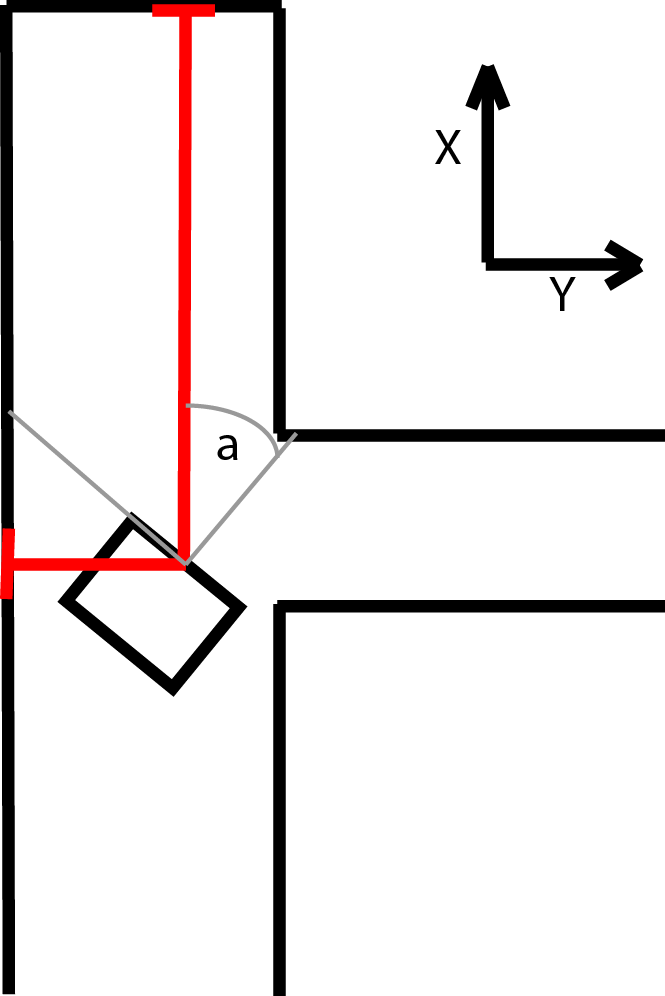
The estimated angle is used to calculate which sensor should point towards the end of the corridor. An interval around the corresponding LRF beam is searched for a local minimum, which should belong to the beam that hits the end perpendicularly. This beam points directly at the end of corridor and is then used to calculate the LRF value for the angle of pico. The difference is calculated between the previous and current distance to the end wall which is the position change for either x or y used in the kalman update. The other position change is calculated in similarly, but in stead of the end of the corridor the distance to the side wall is used. Since it is possible to lose sight of a wall, for instance when driving on an intersection, a safeguard is put in place. If the position change based on the lrf is to big, it is assumed that the LRF data is unreliable for that update cycle and only the odometry data is used. This is done by switching between two R matrices, one of which sets the contributions of the laserdata to zero. In the regular R matrix the contribution of the LRF data is weighed more heavily under the assumption that the LRF is more reliable overall.
Implementation of method
Interface
Retreiving Velocity data
Retreiving Odometry data
Retreiving LRF data
Initializing position
Calculating coordinates from LRF
Implementation of Kalman filter
Technicalities
Integration
.... ....
Experiments
Seven experiments are done during the course. Here you can find short information about dates and goals of the experiments. Also there is a short evaluation for each experiment.
Files & presentations
- Initial design document (week 1): File:Init design.pdf
- First presentation (week 3): File:Group3 May6.pdf
- Second presentation (week 6): File:Group3 May27.pdf
Videos
Experiment 4: Testing the potential field on May 29, 2015.
Archive
This page contains alternative design that is not used in the end. To see what we have worked on during the entiry process, it can be interesting to look at some of these ideas.