Mobile Robot Control 2023 Rosey

Welcome to the group page of team Rosey! This page is currently under construction.

Project organisation

Group members of team Rosey

Name	Student ID
Eline Wisse	1335162
Lotte Rassaerts	1330004
Marijn Minkenberg	1357751
Rainier Heijne	1227575
Tom Minten	1372300
Lowe Blom	1266020

Midterm presentation

During the midterm presentation, team Rosey presented their plan of action to make the robot deliver orders in a restaurant. The slides are available below for comparison to the final product.File:Midterm presentation Rosey.pdf

Work division

The group identified three 'major parts' of the assignment. These are the localisation, the global and local navigation of the robot. The group additionally saw use for an overseeing role, which should ensure that the interfaces between the functions are clear. The work is divided as follows:

• Marijn : System architecture and overview
• Tom : Global navigation
• Eline & Rainier : Local navigation
• Lowe & Lotte : Localisation

System architecture and overview

...

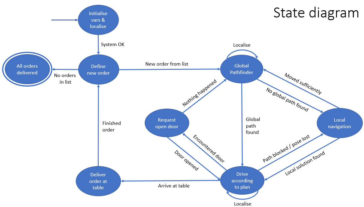
Current state diagram

Intermediate version of state diagram (17-06-2023)

Global Navigation

The global navigation uses the A* algorithm to find the shortest path to from a starting node to a goal node. The A* algorithm uses a predefined grid of nodes. This grid is applied by a JSON file, generated with Matlab. With Matlab, the grid nodes with their connections are manually chooses in the known map. On top of that, we were inspired by the lecture about Safe navigation in a hospital environment to introduce some context-aware navigation into our model, by means of semantics. Each node contains some semantic information about its environment, described by a integer. The following semantic integers are included: 0 = table 0, 1= table 1, ..., 49 = table 49, 50 = door, 99 = empty (meaning no semantic information present). This information is also included in the JSON file.

Preparation phase

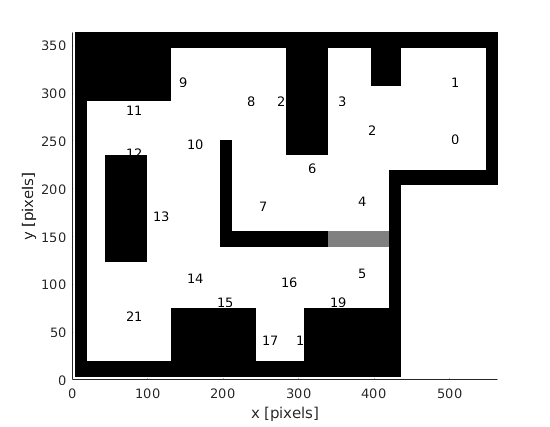
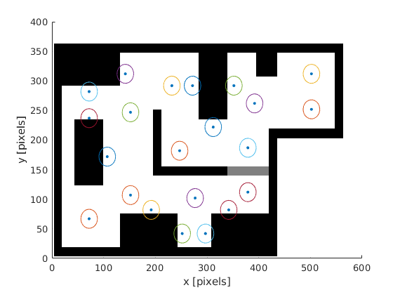
Create a JSON containing the grid information with the Matlab script below. The script has a visualization tool for plotting the position of all nodes. In the next graphs, the locations of the grid points in the final challenge are visualised. The circle has a radius of 20 centimeters. The local navigation assumed that the robot has reached the node when it is 20 centimeters from the node.

The corresponding Matlab script to generate the graphs and the JSON grid file: (click 'Expand'):

%% Data
clear all;
% Points in pixels, personally used pinta for that
x = [500,500,390,350,377,377,310,245,230,140,150,70,70,105,150,190,275,250,295,340,270,70];
y = [110,50,100,70,175,250,140,180,70,50,115,80,125,190,255,280,260,320,320,280,70,295];
% move zero point for matching worldmodel
x = x+2;
y = (y*-1+362);
% scale to meter
res= 1/80; % 80 pixels per meter
x_m = x*res;
y_m = y*res;
%% semantics
% add semantics to certain nodes
% 0: table 0, 1: table 1, ... 49: table 49, 50: door, 99: empty
% also add coordinates of the semantic objects when necessary
sem(1:length(x)) = 99; % fill array with 99 (empties)
semx(1:length(x)) = 0; % fill array with 99 (empties)
semy(1:length(x)) = 0; % fill array with 99 (empties)
sem(10) = 0;
semx(10) = 0.9375;
semy(10) = 4.0625;
sem(12) = 0;
semx(12) = 0.9375;
semy(12) = 4.0625;
sem(4) = 1;
semx(4) = 3.8750;
semy(4) = 3.7500;
sem(7) = 1;
semx(7) = 3.8750;
semy(7) = 3.7500;
sem(21) = 1;
semx(21) = 3.8750;
semy(21) = 3.7500;
sem(13) = 2;
semx(13) = 0.8750;
semy(13) = 2.2500;
sem(14) = 2;
semx(14) = 0.8750;
semy(14) = 2.2500;
sem(16) = 3;
semx(16) = 2.3750;
semy(16) = 0.5625;
sem(18) = 3;
semx(18) = 2.3750;
semy(18) = 0.5625;
sem(20) = 4;
semx(20) = 4.6250;
semy(20) = 0.5625;
sem(19) = 4;
semx(19) = 4.6250;
semy(19) = 0.5625;
doorNodes = [5,6] % door nodes
for i =1:length(doorNodes)
sem(doorNodes(i)) = 50;
end
%% connections
% define connections for each node, using input mode of matlab
conn_challenge_restaurant = zeros(length(x),10);
for i = 1:length(x)
i
prompt="type Connections, in form [a,b] when more connections exists: "
output = input(prompt)
for j = 1:length(output)
conn_challenge_restaurant(i,j) = output(j)
end
end
%% Plot
close all;
figure()
text(x, y, string((1:numel(x))-1)); % python numbering (index 0:..)
%text(x, y, string((1:numel(x))-0)); % matlab numbering (index 1:...)
axis([0, 564, 0, 364])
hold on
% visualise bitmap with points
I = imread('RestaurantChallengeMapRotatedFlipH.png');
h = image(2,2,I);
uistack(h,'bottom')
% size of points, which forms the circle around node
sm = 10;
% radius of circle about node
R = 16; % 0.2*80, 20 centimeter radius
th = linspace(0,2*pi) ;
figure()
scatter(x,y,sm,"filled")
hold on
for i = 1:length(x)
x_c = R*cos(th)+x(i) ;
y_c = R*sin(th)+y(i) ;
scatter(x_c,y_c,1,"filled")
end
I = imread('RestaurantChallengeMapRotatedFlipH.png');
h = image(2,2,I);
uistack(h,'bottom')
%% generate JSON
S.nodes = struct("x", num2cell(x_m), "y", num2cell(y_m), "semantic",num2cell(sem),"semanticX",num2cell(semx),"semanticY",num2cell(semy))
S.connections = conn_challenge_restaurant
s = jsonencode(S,PrettyPrint=true)
if exist('grid.json', 'file')==2
prompt="do you want to remove old grid.json file? (y=1/n=0) "
output = input(prompt);
if output == 1
delete('grid.json');
disp("Caution, old grid.json file is deleted...")
end
end
fid=fopen('grid.json','w');
fprintf(fid, s);
disp("new grid.json is succesfully saved")

Initiation phase (run once)

The json file is imported with the loadConfigFile()and the grid is constructed withconstructGrid().

Global path finder phase

In globalNavigation(), there are a few steps which has to be taken for determining the best path as node sequence.

1. First, the robot determines its own position in its map and the closest node is found. One assumed that there is no complete blocking object as a wall in between the robot and the closest node, i.e. sufficient nodes has to be properly placed.
2. The goal node is found by finding the corresponding semantic number of the destination table
3. The aStar()is executed to find the best path - In case the output is [-1], there is no path available with the provided information. Possibly causes: connections are not correctly defined are essential connections are removed. - the output with the sequence of nodes to (and including) the goal node is written to the global*pathNodeIDsvariable
4. The main function returns whether a path is found

Cutting connections in case of blocking objects or close doors

---Write when local navigation is finished---

Local Navigation

...

Localisation

...

Testing the software

Final challenge day

...