Embedded Motion Control 2014 Group 6

Wout Laarakkers 0828580

Rik Boonen 0805544

Dhruv Khandelwal 0868893

Suraj Prakash 0870060

Hans Reijnders 0806260

Updates

• Include Bool action_done and Bool wall_close in topic drive for handshake (23 May)

Planning

Week 1 (2014-04-25 - 2014-05-02)

• Installing Ubuntu 12.04
• Installing ROS
• Following tutorials on C++ and ROS.
• Setup SVN

Week 2 (2014-05-03 - 2014-05-09)

• Finishing tutorials
• Interpret laser sensor
• Positioning of PICO
• having ore first meeting

Week 3 (2014-05-12 - 2014-05-16)

• Programming corridor competition
• Corridor competition

Week 4 (2014-05-19 - 2014-05-23)

• Creating basic structure for programming in Ros
• Planning
• Dividing tasks

     * Drive node: Dhruv Khandelwal
     * Decision node: Hans Reijnders, Rik Boonen
     * Arrow node: Wout Laarakkers

• Programming individual parts

Week 5 (2014-05-26 - 2014-05-30)

• Programming individual parts
• Testing parts
• Integrating parts

Week 6 (2014-06-02 - 2014-06-06)

• Programming individual parts
• Testing parts
• Integrating parts
• Deadline for the nodes

Changes in group

Unfortunately Suraj Prakash has decided to quit the course, because he doesn't has enough time.

Corridor competition Software design

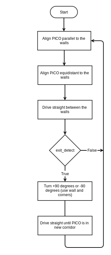
Global Software design

Design Goals

for ore global software we had 3 design choices
1.Split in to equal parts
2.Make logical sense
3.Individual testable

To accommodated this design we came up with a global software design that exist out of 3 nodes.A drive node that does all the driving like a car driver would do. Derision node, This would make all the decisions and would tell the drive node what action to execute. Arrow , would tell the decision node if it sees a arrow so it can take it in consideration for the next decision. This design is based on a real life situation where a driver(drive node) listens to his car navigation (derision-node). witch is constantly updated with the latest traffic information (arrow-node).

This software makes logical sense and is very good individual testebel.

Drive-node: can use numpad to input what situation the dissension node would send to him
Decision-node: can drive around whit teleop to see if it detects the correct situations and makes the correct decisions
Arrow-node: bag file's

The strong part of this design is the individually testebel parts and the logic structure of the software.

Structure

The first draft of the structure of nodes and topics is shown below.

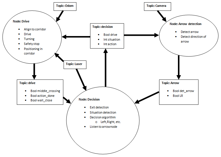
The integer 'situation' and 'action' have certain values corresponding to different cases. These cases are defined as shown below.

Situation
1	Detected corridor
2	Detected dead-end
3	Detected corner right
4	Detected corner left
5	Detected T-crossing (right-left)
6	Detected T-crossing (right-straight)
7	Detected T-crossing (left-straight)
8	Detected crossing
9	Unidentified situation

.

action
1	Stop
2	Straight
3	Right
4	Left
5	Turn around
6	Follow left wall
7	Follow right wall

Taking corners

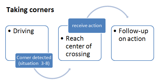
Decision node

The decision node is designed to act like a navigation tool. It tells the drive node where to go, it has to publish which situation pico is approaching and which way pico has to go. So, for example: T-junction up ahead and go right. In order to do this the decision node first has to detect which situation pico is approaching. Then it has to decide which way to go. We will first look at the Situation determination and then look at the Action determination (telling which way to go).

Situation determination

To detect a situation 2 methods have been used. The first method focuses on sending the right situation and not making errors, but is slower in giving the situation. The second method will give the situations earlier, but will make some more errors. We will first look at method 1, its algorithm, simulation/test results and conclusion. Then we discus method 2 also including its algorithm and simulation/test results and give a conclusion.

Method 1: Situation determination

In order to determine which situation we are approaching, we want to know 3 things: is there a corner to the left, is there a corner to the right and can we go straight ahead?

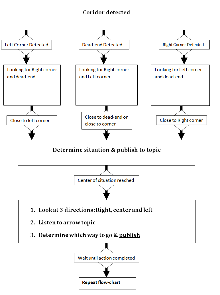
We determine these 3 things by using the laser data. Unfortunately we will not always detect the corners and dead end at the same time, so when we detect one of these 3 we will drive to a fixed distance from the situation. In this time we drive we will determine if we also find the other two characteristics of the situation. Using the information we have we can determine the situation and publish it on the topic.

The flowchart shown below shows the steps in this algorithm. Also there is an example situation to clearify the algorithm better.

Flowchart

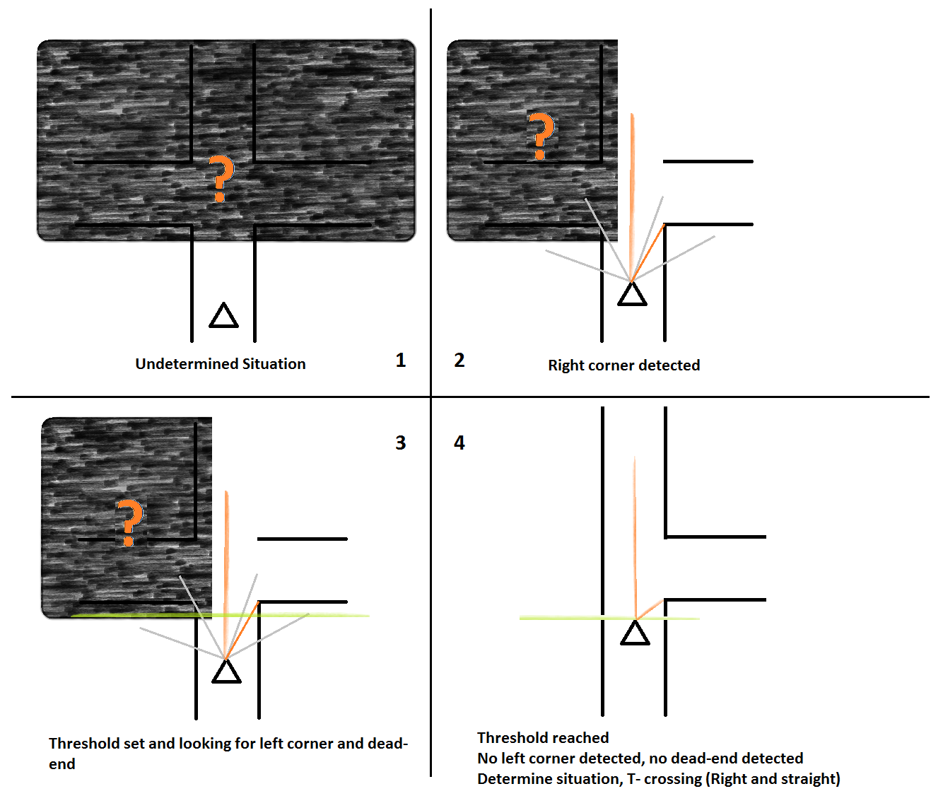
Example

In the Example below we see:

In picture 1: Pico approaches an unidentified situation.

In picture 2: Pico has detected a right corner, this could mean that the next situation is a corner to the right, but pico is not sure if there is a corner to the left and if we can go straight ahead.

In picture 3: Pico has set a threshold, meaning that when reaching the threshold pico will give the situation it has detected. In the time driving towards the threshold pico will look if there is a corner to the left or he can go straight ahead.

In picture 4: Pico has reached the threshold and has seen that he can go straight and to the right. So the node will send situation 6.

Simulation Results

To test this algorithm in simulation we used a few methods.

First one was to put in pico in a maze and let it detect a situation and not use the drive node, because the drive node was not yet ready. This worked very well. Although there were some minor flaws.

One flaw is that a situation like a T-junction where pico can go straight and left or right and the straight had dead-end, then this algorithm detects a corner. During first simulations this did not look like an problem, but later it showed the drive node could not handle with this.

The second method was to combine the drive node and the decision node. Now we saw that the drive node could not handle the flaw as stated above. Also the situation often came to late to the drive node, and the drive node could not make sure to see the turn and act on it.

Test Results

Testing the decision node with the real pico we noticed a few things:

1. The distance to a corner is not reliable, so the threshold is not used correctly

2. If the situation and threshold is used correctly then the situation is to late and the drive node cannot make sure a good turn.

Conclusion

This algorithm works well without the drive node. There are some flaws like the unreliable distance and the dead-end detected at a T-crossing with dead-end, but these problems can be solved without changing the overall algorithm to much. The real problem is that of giving the situation late. This is a main characteristic of this algorithm, giving the situation later but not making mistakes.

To solve this problem either the drive node or the decision node had to change. We chose to change the decision node and create a new algorithm for the situation determination. This new algorithm is described in Method 2.

Method 2: Situation determination

This second method has been made, because in method 1 the situation was send to late. Where in method 1 the focus was on not making errors, here the focus lies more on sending the next situation early. This works better when combining this node with the drive node, because when a situation is detected (perhaps only a right corner of a T-junction) then the drive node can already start looking for a right corner. Maybe this can be seen as the driver in the car that knows where to look for and then finds it faster.

Situation counter

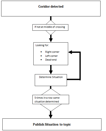
When sending every detected situation, false or right, we noticed that the situation is mostly right and sometimes wrong. Inorder to get rid of most of these falsely determined situation we added a counter. This counter will only publish the situation if there is 5 times the same situation detected.

Action determination

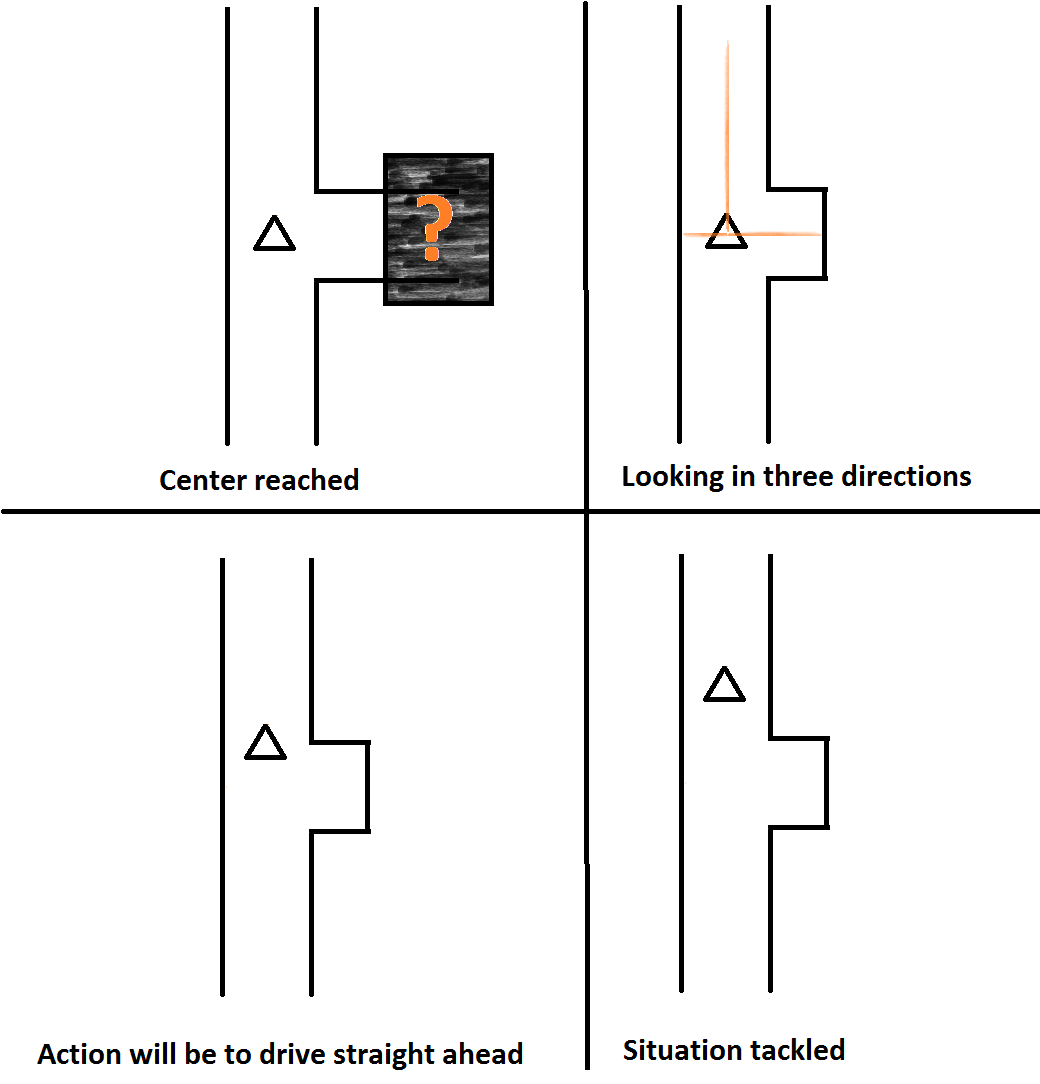
When we have published a situation, then the drive node makes sure we drive to the center of the situation. If we are in the center, we will determine if there are deadends in any turns, look if there are any arrows and then make a decision which way to go.

Example

Drive Node

The drive node is designed to operate like the driver of a car. The Decision node provides localalized information about the current situation to the Drive node, which drives Pico to the centre of the situation. The Decision node can then make a better choice of the action required. After recieving the action from the Decision node, the Drive node performs the action, and then listens to the Decision node for the next situation.

The Drive node listens to the Decision topic, the Laserdata topic and the Odometry topic to perform it's various functions. The Drive node consists of many small modular functions that perform specific tasks, such as driving straight with a specified velocity, performing a left turn, and so on. These small fuctions are called repeatedly and in an ordered fashion to perform the action suggested by the Decision node.

Reaching the middle of a corner/crossing

The Drive node includes a corner detection algorithm, that allows it to drive Pico to the centre of a corner/crossing. However, while testing, we realized that detecting the corners alone was not sufficient to drive to the centre of a corner/crossing, due to the limited range of the laser data. Hence we included data from the Odometer to make this action more reliable. Thus, the node uses laser data to look forward and odometer to look back to reach the middle.

The Drive topic

The drive node publishes on the cmd_vel topic and the drive topic. The drive topic consists of the following flags:

• action_done
• wall_close
• middle_reached

These flags inform the Decision node the position of Pico in the maze. The wall_close flag informs the Decision node that Pico is very close to a wall. The middle_reached flag informs the Decision node that Pico has reached the middle of the conren/crossing, and that the Decision node should make a decision on the action. The action_done flag informs the Decision node that Pico has completed the action and that the Decision node should start looking for the current situations again.

Safe Drive

The Drive node is also responsible to ensure that Pico does not run into a wall. The node does this by checking all the laser data distances. If a wall is detected withing 30 cms, all motion is stopped and Pico is subsequently aligned to the corridor and driven to the center of the corridor's width. All actions are then resumed.

Aligning

Our software structure relies heavily on the fact that Pico will be able to align itself when it is in a coridor. This allows better sitaution determination for the Descision node and also allows the drive node to drive Pico to the middle of a situation once the situation is determined. Hence, we decided to implement a two fold alignment algorithm which aligns Pico parallel to the two walls of a corridor and also drives Pico to the lateral center of the corridor.

To align parallel to the walls, we implemented an algorithm similar to a gradient ascent algorithm. We use the laserdata values to calculate the gradient around the 0 degrees direction, and then turn Pico along the positive gradient until the laser range at 0 degrees hits a maxima. The algoithm is illustrated in the figure below.

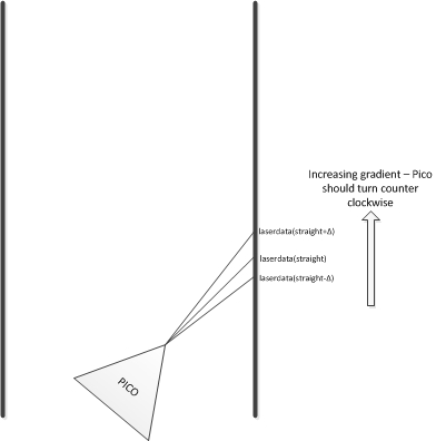
The algorithm described above turns Pico such that it faces the longest direction when it is in a corridor, and hence this algorithms fails if the error in Pico's direction is more than 90 degrees. However, we do not expect such a large error to occur during the maze competition. Another weakness of this algorithm is that when Pico is close to the end of the corridor, this algorithm will make Pico turn towards the corner of the corridor and not straight ahead, as shown in the figure below:

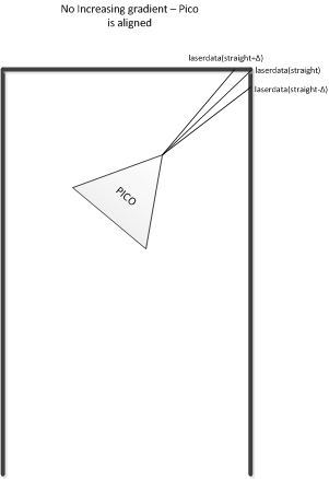
To correct this error, we implemented another algorithm which aligns Pico parallel to the walls by comparing the distances on the left and on the right of Pico. The algorithm is illustrated in the figure shown below:

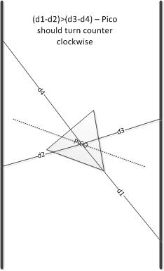
To check if Pico is at a tilt compared to the walls of the corridor, we calculate the distances (d1-d2) and (d3-d4), and if these distances are of opposite signs, i.e. if (d1-d2)*(d3-d4)<0, Pico can be aligned further. To make the algorithm robust, some tolerance values were used for the comparison. While this method of aligning Pico worked in simulation, we decided not to include it in the software for the final maze competetion as we did not get a chance to test this on the actual hardware setup.

Aligning Pico to the center of the corridor is much simpler; we simply measure the distance to the left and right of Pico, and move Pico laterally until the distances are within a tolerance range of each other.

Before using these alignment techniques, the drive node first checks whether Pico is in a corridor as these algorithms will fail if Pico is in, for example, a corner or a crossing.

Function Description

A breif description of the functions created to perform the modular tasks is given below. The flow of logic in the node will be explained using these function names.

• align_parallel(): This function uses the laser data to align Pico parallel to the two walls of the corridor it is currently in. This fuction uses an adapted form of a gradient ascent algorithm.
• align_center(): Once Pico has been aligned parallel to the walls, this function is used to bring Pico to the center of the corridor.
• driveStraight(): This fuction drives Pico straight.
• turnAround(): This function turns Pico by 180 degrees. It integrates the pose values of the odometry sensor until the result is pi.
• turnLeft(): This function turns Pico by 90 degrees to the left.
• turnRight(): This function turns Pico by 90 degrees to the right.
• reachMiddle_right(): This function allows Pico to reach the middle of a right hand corner. Here, a distinction has been made between a right hand corner and a right-straight T crossing. This function does not make use of corner detection.
• reachMiddle_right_T(): This function allows Pico the reach the middle of a T-crossing with a right exit. It makes use of corner detection.
• reachMiddle_left(): This function allows Pico to reach the middle of a left hand corner. Here, a distinction has been made between a left hand corner and a left-straight T crossing. This function does not make use of corner detection.
• reachMiddle_left_T(): This function allows Pico the reach the middle of a T-crossing with a left exit. It makes use of corner detection.
• stop(): This function stops Pico.
• detectCornersLeft(): This function detects corners on the left side of Pico, i.e from 0 degrees to 120 degrees.
• detectCornersRight(): This function detects corners on the right side of Pico, i.e from 0 degrees to -120 degrees.

Sequence of Actions

Based on the situation and the subsequent action recieved by the Drive node, the sequence of actions performed by the Drive node is shown in the table below.

Situation vs. Action

	Default	Action 1	Action 2	Action 3	Action 4	Action 5
Situation 1	Align	stop	drive Straight	Error	Error	Error
Situation 2	-	stop	Error	Error	Error	turn Around
Situation 3	reach middle of corner	stop	Error	turn right and finish corner	Error	turn Around
Situation 4	reach middle of corner	stop	Error	Error	turn left and finish corner	turn Around
Situation 5	reach middle of T junction	stop	Error	turn right and finish corner	turn left and finish corner	turn Around
Situation 6	reach middle of T junction	stop	drive Straight	turn right and finish corner	Error	turn Around
Situation 7	reach middle of T junction	stop	drive Straight	Error	turn left and finish corner	turn Around
Situation 8	reach middle of crossing	stop	drive Straight	turn right and finish corner	turn left and finish corner	turn Around

Flowchart

For better illustration, a flowchart depicting the flow of clogic for the first 4 situations (corridor, dead-end, right corner and left corner) is shown below:

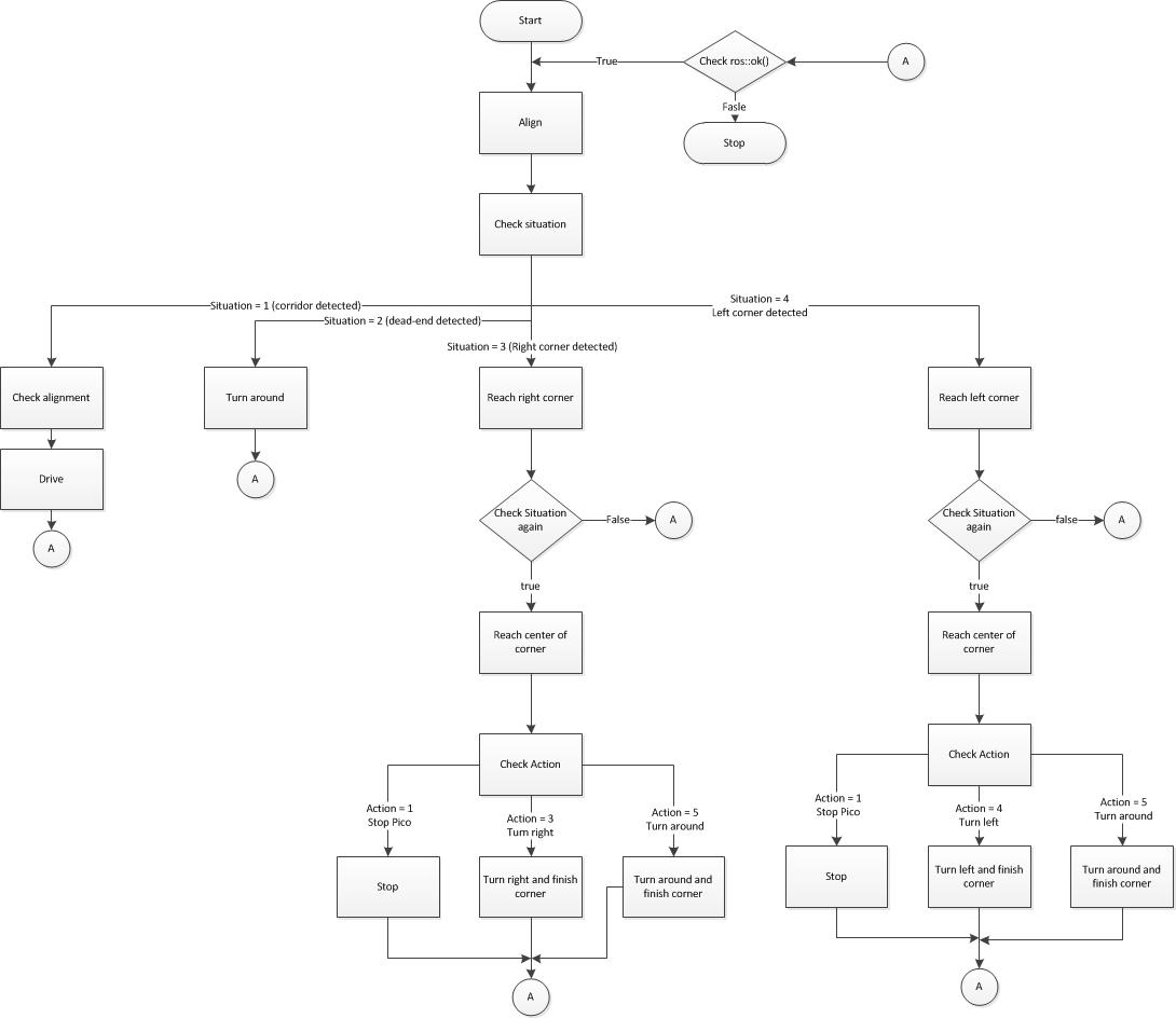
In an earlier design, the software was integrated in such a manner that the drive node would act as soon as it recieved a situation from the decision node. This was not a good idea as the first situation determined was not always the right situation. Hence we changed the nodes such that they would communicate with each other once before just before Pico reaches a corner. At that instant, the Decision node can identify a more accurate situation.

Novelty of the Drive node

From what we saw in the maze competion, not all teams aligned Pico to the corridors, most of the teams used algorithms in which Pico was repelled away from the walls. We found aligning Pico to the walls of a corridor a more intuitive way of implementing our drive node. As our software structure is inspired by a car driver-navigation system, we chose to design the drive node such that it would imitate a car driver. While driving a car, we instinctively tend to align the car to the road, and this is what we tried to replicate with Pico.

Another part of the drive node that we were particularly happy about (until one week before the maze competition) was the turning. We used the odometer to turn Pico through specific angles, and the results were very reliable. Unfortunately, a couple of days before the maze competetion, we found out that the turning algorithm almost never works on the actual hardware. We had a word about this with _________, who suspected a fault in the encoder. However, it was too late to make any changes to the hardware setup. Thus we had to completely change the turning part of the drive node one day before the maze competition.

Arrow Node

The arrow node is made for detecting a arrow and its orientation of a arrow when asked by the information node. The info this node publishes then helps the decision node decide what turn to take.

Design of Arrow-node

the main design decision in the arrow node is based on the use of hough transform. this transformation in combination with the line detector tuned correctly make us able to so arrows of any distance. This would benefit the arrow detection because the exact distance to the arrow is unknown and variances between each maze. Also the custom flood fill that is being used had a much better result that the standard flood fill of the opencv library

Convert image to hsv

First the camera rgb camera image is converted to a hsv image. this for making the following step easyer

Threshold image

The image is now threshold so that only the red parts of that would be red in a rgb picture become wit and the rest black (a binary image)

Custom flood fill

A flood fill is used to fill in the small imperfections in the arrow and also make the edges of the arrow smoother. This custom flood fill also removes "alone" pixels that can be in the image from the camera noise

Blur the image

The binary image is blurred to make the edges even smoother for the next step.

Canny edge detector

a canny line algorithm is used to detect the outer lines of the arrow image

Detect lines

The lines are then detected by using a Hough transform algoritm

Calculate line gradients + position

The lines are filtered so only left 2 and right 2 lines are saved. For these 4 lines the gradient is calculated with the following formula
[math]\displaystyle{ \nabla = \frac{y_{1} - y_{2}}{x_{1} - x_{2}} }[/math]
By looking the gradient and the postion of the lines the direction of the arrow can be calculated

Calculate the direction

by letting the above steps happen for 2 seconds and save how many time there was a arrow left right and no detected it can be sad if there is a arrow.