Embedded Motion Control 2014 Group 1

Introduction

This wiki page is written as a report for the course Embedded Motion Control (EMC). For this course software needs to be written for a robot (PICO) to autonomously solve a maze. As an intermediate review the robot has to drive through a corridor and take the first exit.

This page aims to give all relevant information with respect to the EMC course. First the approach to solve the maze is explained. Second all software components are explained. Furthermore the result of the corridor challenge and maze competition are described. Last conclusions and recomendations are drawn.

For organizational information as planning, meetings and group info there is referred to the appendix. The appendix also shows all the videos made in simulation and with experiments and a summary is given of all messages used for the communication between the ROS nodes.

Approach

In this section the considerations with respect to the choice of a maze solving algorithm are explained. Furthermore the software architecture based on the chosen maze solving algorithm is presented.

Considerations

Solving a maze can be done in different ways. For the maze competition the following algorithms are considered:

• Random mouse algorithm
• Wall follower
• Pledge algorithm
• Tremaux's algorithm
• Dead-end filling
• Recursive algorithm
• Shortest path algorithm

Explanations about these algorithms can be found at: algorithms.

Our approach for the maze competition will be based on the wall follower. With additions to the wall follower as arrow detection and dead-end recognition the maze can be solved in a simple, efficient and robust way. The choice for this algorithm is based on the fact that its simple, easy to program but nevertheless effective.

The starting point of this algorithm is that the mobile robot starts following passages and whenever a junction is reached it always turn right (or left). Equivalent to a human solving a Maze by putting their hand on the right (or left) wall and leaving it there as they walk through. This algorithm will be improved by adding arrow detection and dead end recognition.

Examples of a maze solved by the Wall follower algorithm are shown below.

• Link 1
  
• Link 2
  

Implementing a wall follower algorithm can be done in different ways (see below). The choice of implementation was based on the following defined requirements:

• The algorithm needs to be modular, i.e., it must be possible to start with a simple algorithm which can be improved by adding and deleting different nodes or parts of code.
• The wall follower algorithm needs to be as robust as possible to be able to cope with the defined situations of the maze but kept as simple as possible.

For the implementation different approaches are considered. First it is decided how situations are recognized and decisions are made. Furthermore it is determined with what approach PICO is given its trajectory.

Situation recognition/Decision making
To recognize situations and act on them some kind of a representation of the world is necessary. This is also needed to localize PICO. Three approaches are considered for the wall follower algorithm.

The first approach is mapping of the environment with gmapping. Gmapping makes it able to Simultaneous Localize And Map (SLAM). Based on this map and localization it is able to plan a path in the environment. Advantage of this approach is that gmapping is a often used ROS package which only needs tuning to use it. Furthermore it is possible with a map to have a robust representation of the environment. The main drawback of this approach is that the biggest advantage of a map is not used. When a map is known before hand a motion planner can determine the fastest route to the exit of the maze. Unfortunately this is not the case with the maze competition. Furthermore within the time span of the course mapping can be a to complex and time consuming approach.

The second option is situation recognition based on laser data. With use of laser data it is possible to determine the position of the robot with respect to the walls. Furthermore it is possible to detect exits and dead end based on laser data. Laser data is very easy to interpret because if gives straightforward geometrical information. Though the drawback of laser data is that it is not very robust. Noise can be encountered and give unpredictable results. Also, it is difficult to see an exit in advance solely based on the laser data.

The last option is recognizing situations based on lines. With use of a hough transform lines can be determined based on the laser data. These lines will represent the walls in the case of the maze competition. Line data is more robust then laser data for situation recognition. Also it is easier to determine if there is an exit ahead or a dead end. Difficulties with line detection are problems with the output of the line detection. It can be the case that multiple lines are given for one wall or that a line is drawn where no wall is. This has mostly to do with correct tuning of the algorithm.

As already stated in the requirements the algorithm will be build as a modular design to start simple and improve the algorithm during the course. Because of this reason there will be started with laser data to recognize situations. The final goal is to use Line detection in the software architecture. Gmapping is not chosen because is it seen as a more difficult and time consuming approach then necessary for the maze competition. Our goal is to use the time for a robust algorithm with use of laser data and later line detection.

Behavior
Based on the laser or/and line data situations can be recognized. Though PICO still needs to get commands what his trajectory will be. This can be done in a global and local way. Global planning is planning a path in advance. Local planning is determining a path based on the current sensor data. Because no map is made (see section above) local planning is used.

For the local planning it is decided to use a state machine. Based on the situation the behavior of PICO is determined. The state machine will be used in such a way that different states can be added during the course. A modular and robust design are again two of the most important requirements for the state machine.

Software architecture

In the previous section it is determined that for situation recognition line detection and laser data will be used as an input. For the behavior determination a state machine will be used. These different operations will be implemented in ROS. Because of the requirement to be able to have a modular design the different operations will be split in ROS nodes. This will result in a good overview of the system architecture and a modular design where it is able to add and delete different nodes in an easy way.

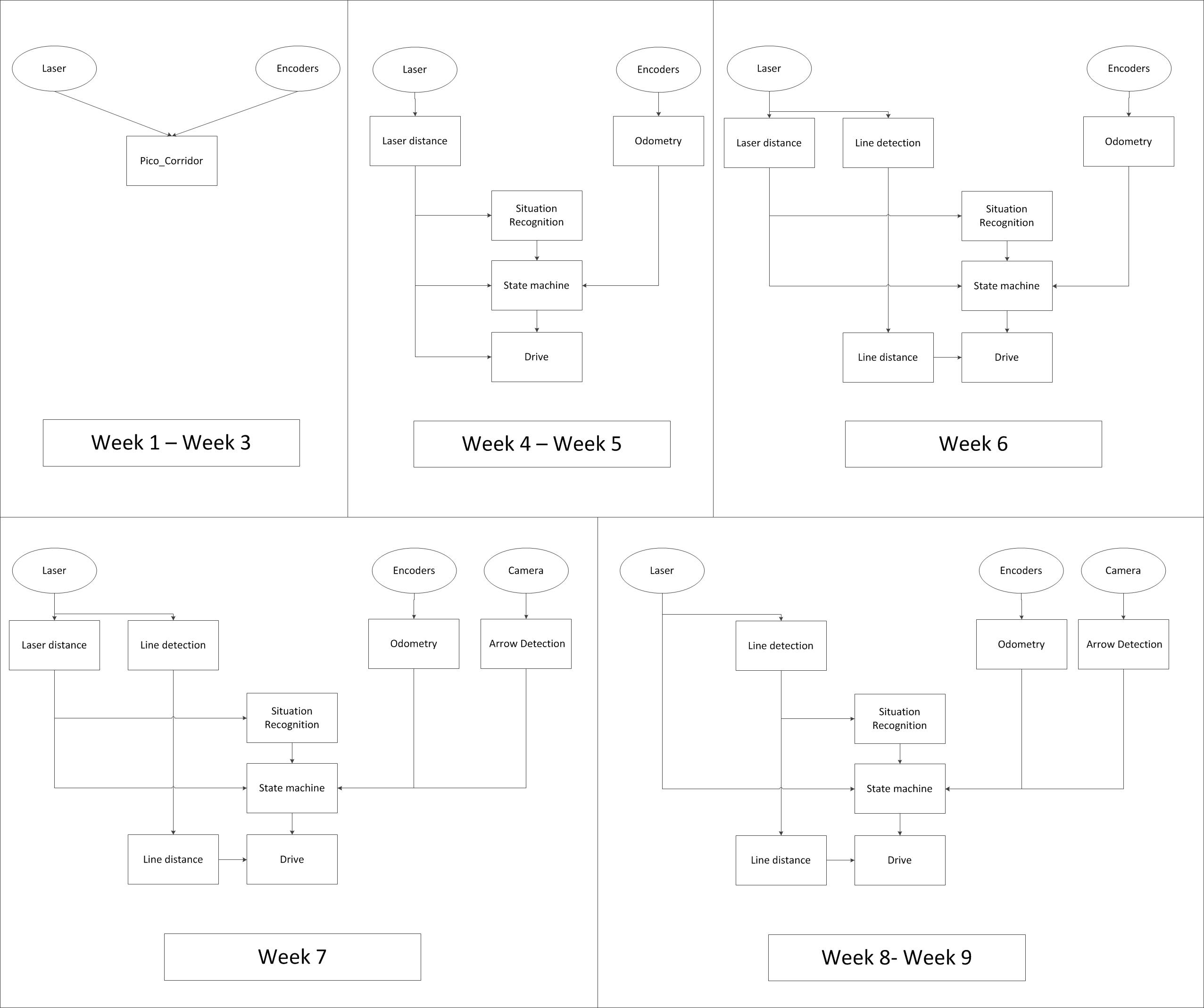
The figure below shows how the software architecture changed during the course (click on picture to enlarge). Eclipse blocks represent sensor data and rectangular blocks represent ROS nodes. The first three weeks one node is used for the corridor challenge. After this the new architecture was implemented and improved over the weeks. Most important are the addition of the line and arrow detection. Furthermore it becomes clear that the line detection replaced the laser distance node. The raw sensor data is only used for safety in the state machine.

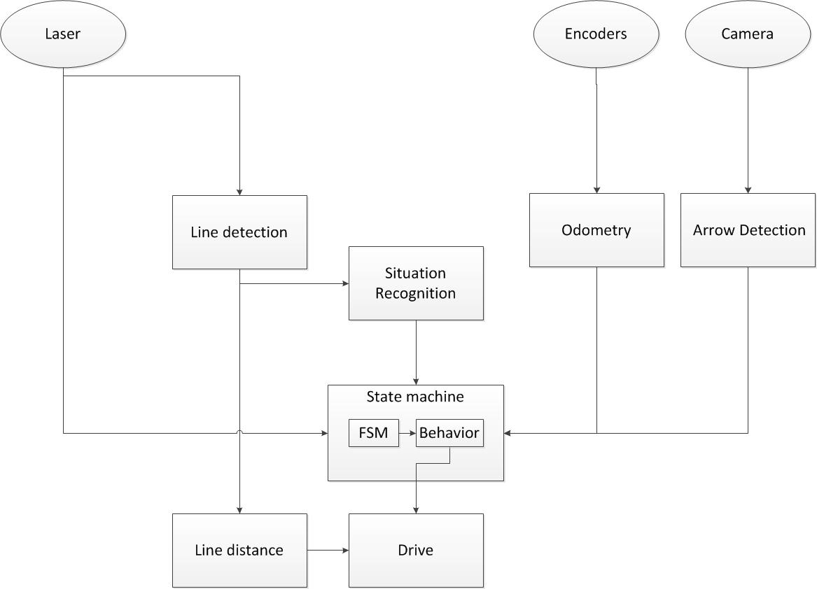
The final software architecture is a robust, modular, simple and logical design. An enlarged picture of the final software architecture is shown below. The working principle in general will first be explained. In the next section the different blocks will be explained in more detail.

Based on the incoming laser data from PICO lines are generated with use of a hough transform and a custom build filter. With use of the line data situations are recognized like exits and dead ends. This information is send to the state machine. Next to the situation recognition also information about a detected arrow is send to the state machine, this gives simply information if there is an arrow to the left or right. Whit this information it is determined what kind of behavior is needed in the given situation. An example could be that the robot needs to turn 90 degrees to the right because a t-junction is recognized. The state machine sends the command to rotate the robot with a given speed until the odometry shows that the robot has turned 90 degrees.

The needed behavior of the robot is send to the drive process which sends the velocities to PICO. The drive block also makes sure that the robot drives in the middle of the maze corridors and has an orientation perpendicular to the driving direction. This is also done with the line input. Dependent on the state of the robot this control is on or off.

The raw laser sensor data is used for the 'safe drive' state of PICO. When an object is detected on a certain threshold PICO will go to its safety state.

Software Components

Line detection

The primary sensor for gathering information about the environment of PICO is its laser scanner. The scanner describes a discretized 270-degree angle around PICO, in the plane of the scanner, in the form of polar coordinates of the closest detected points. While useful in some cases, this results in large dataset from which it can be difficult to extract useful information, such as the distribution of walls surrounding PICO or an upcoming dead end. Since the environment will be built entirely of approximately straight walls, a logical step is to transform the laser points to a set of lines representing the walls. This greatly reduces the number of coordinates, allowing for a better interpretation of the surroundings.

Goal

The goal of this component is to accurately transform received laser points to lines describing the surrounding walls. Lines will be described by four Cartesian coordinates.

Considerations

For detecting straight lines, a commonly used method is the (generalized) Hough transform. The Hough transform is an algorithm which detects points in an image which together form a straight line. It does this by collecting sets of neighboring points, each of which could be a point on the same straight line. If a large enough set of such points is found, a line is ‘detected’. A drawback of using the Hough transform for this application is that it cannot immediately be used on the laser scan data, because the Hough transform requires an image to operate on. This requires the collected laser scan data to be transformed into a binary image on which the Hough transform can be applied, while the resulting lines too need to be transformed back into real-world coordinates. Another way to collect lines from the laser data would be to write a simplified algorithm which doesn’t require an image, but operates directly on data from the laser scan. Such an algorithm could use the fact that the laser data is ordered in increasing angle and could look at consecutive points with similar X and Y coordinates. However, after discussion the decision was made that a self-written algorithm would be too complex to develop if it is to be robust in varying situations. In contrast, the Hough transform has been thoroughly developed over may years and therefore delivers a more generalized solution. The decision was therefore made to use the Hough transform for detection of lines.

Implementation

In c++, the Hough transform is implemented in the OpenCV library through the HoughLines and HoughLinesP functions. These functions operate on a binary image (cv::Mat object). In order to arrive at such an image, several transformations are performed:

• From laser scan points in polar coordinates (sensor_msgs::LaserScan) to Cartesian points (sensor_msgs::PointCloud2). This is done using ROS's built-in projection method laser_geometry::transformLaserScanToPointCloud(), which transforms the laser scan to points in a fixed frame, in this case PICO's base (/pico/base_link).
• From PointCloud2 to pcl::PointCloud<pcl::PointXYZ>, which has an easier interface for extracting the individual points. This is done using the the pcl::fromROSMsg() method.
• From points in Cartesian coordinates to a binary image (cv::Mat). This is done by scaling the coordinates and overlaying them onto a matrix of dimensions, which are determined by the chosen resolution and a maximum range. Points are then ‘drawn’ onto the image, resulting in a black-and-white image where each projected point is colored white.

The Hough transform can then be performed on this image, the parameters of which are discussed later. The resulting line coordinates, which are scaled on the dimensions of the image, are then transformed back into real-world coordinates. In order to easily publish them on a ROS topic, and to visualize them in rviz, they are stored in a visualization_msgs::Marker object, containing a list of couples of points describing the lines.

After implementing the Hough transform, it was found that the resulting set of lines contained many small line segments as well as close and approximately parallel lines. It was found that a cause for this was the variance in the coordinates of the detected laser points. Because of this ‘spread’ of the points, several similar lines could be drawn in the same area, whereas only a single wall exists. Several solutions were investigated, such as further tuning of the parameters of the Hough transform and the use of blurring and edge detection on the input image. However, these solutions often resulted in decreased accuracy, many short line segments or did not fully solve the problem. Therefore, a different approach was pursued, in the form of a custom filter to combine multiple ‘duplicate’ lines into a single line.

Custom filter

For two lines to be considered to form a single line in the real world, they must meet some conditions:

• Their angle must be identical up to a threshold (here +/- 10 degrees)
• The distance perpendicular to the lines must be identical up to a threshold (here 0.1m)
• The lines must overlap along their length, or the distance between the endpoints must be within some threshold (here: 0.1m)

An algorithm was written to procedurally consider which line segments from a set satisfy these conditions. Matching line segments were then used to determine a single line which best represents them. The algorithm works in the following way:

• The angle of each line segment w.r.t. the origin is determined using theta = atan2(y2-y2/x2-x1). The angle is normalized to the [0,pi] range so that lines in opposing directions are not treated as having different angles. The normalized angles are stored in a vector with the same indices as the line segments for later reference.
• Iterating over the angles, the indices of lines whose angle corresponds to the angle of another line are stored in a new vector. This results in vectors with the indices of approximately parallel lines.
• The original line segments are rotated about the origin by their angle so that they are parallel to the X-axis. Because lines with a similar angle are rotated by the same angle around the same point, their relative distance remains approximately the same.
• The lines are ordered in increasing ‘leftmost’ X-coordinate to facilitate future operations.
• Iterating over the vectors of parallel lines, the distance w.r.t. the X-axis is compared. If the difference in distance between two lines exceeds the defined threshold, the index of the second line is moved to a new vector. This results in new vectors with the indices of lines which are parallel as well as close to each other.
• Iterating over the new vectors, the distance between the rightmost vertex of a line and the leftmost vertex of the next line is determined. If this distance exceeds the threshold, the indices of the remainder of lines are moved to a new vector.
• The result of the previous steps is a set of vectors with indices of line segments which satisfy the conditions to form a single line. For each of these, the minimum and maximum X-value and the average theta and Y values are determined in the rotated coordinate frame. A new line with these coordinates is created, which is rotated back by the average theta value. This line now represents the combination of the original line segments.

Testing of the filter revealed that the new representations matched the position of original laser points very accurately, while reliably reducing the number of lines to the minimum for each situation without falsely removing lines of interest. Because of the effectiveness of the filter, the parameters of the Hough transform could be tuned to allow more sensitive detection of lines, which normally results in more separate line segments, but which are now combined into a single line regardless. This especially improved line detection accuracy for larger distances.

Even though the filter is somewhat complex, it was found to execute computationally efficiently. Because it iterates over relatively small vectors and effectively only executes floating point comparisons, little load is added to the computationally more expensive Hough transform. This means that the filter can be freely applied if the Hough transform is already being used.

While the filter performed accurately for static situations, it was found that during moving, the line representations would slightly vary between frames, in particular the angle of the lines. An explanation for this could be an inaccuracy in the algorithm, which averages the angle of similar lines. Many small line segments with small deviations in angle can therefore pollute the calculated average. One way to solve this would be to calculate a weighted average based on the length of the line segment. As it turned out, however, the relatively small ‘flickering’ of the lines did not cause problems in the relevant control processes, therefore no effort was put into developing this solution.

Because the filter by nature does not depend on any particular process it is used in, it was structured as a static method in a container class. This allows the filter to be re-used by other processes if desired, as will be discussed in the section about Arrow detection.

Conclusion & Recommendations

Combining the Hough transform and a custom filter to the laser scan data, a minimal set of lines is accurately detected within a range of 3 meter. The minimal representation allows for easy use in other processes, such as determining distance to walls and situation detection.

Improvements could be made to the range up to which lines are accurately detected. However, considering the choice for local planning only, the range was found to be sufficient and this was not pursued. Improvements could also be made to the filter to reduce ‘flickering’ of lines in dynamic situations. Finally, line detection as described here is limited to straight lines only, which limits its use in a generalized environment.

Distance

Goal

The goal for this part is to determine the distance to wall to left, right and front wall. Also determine the angle theta with respect to the walls left and right

Considerations

Two different approaches where used to determine the distance to the walls. The first approach was based on the laser data points (laser distance) and the second approach was based on the lines (line distance) generated by the line detection node. The laser distance node was used in the corridor challenge but it was replaced with the line distance node in the final maze challenge

Laser distance

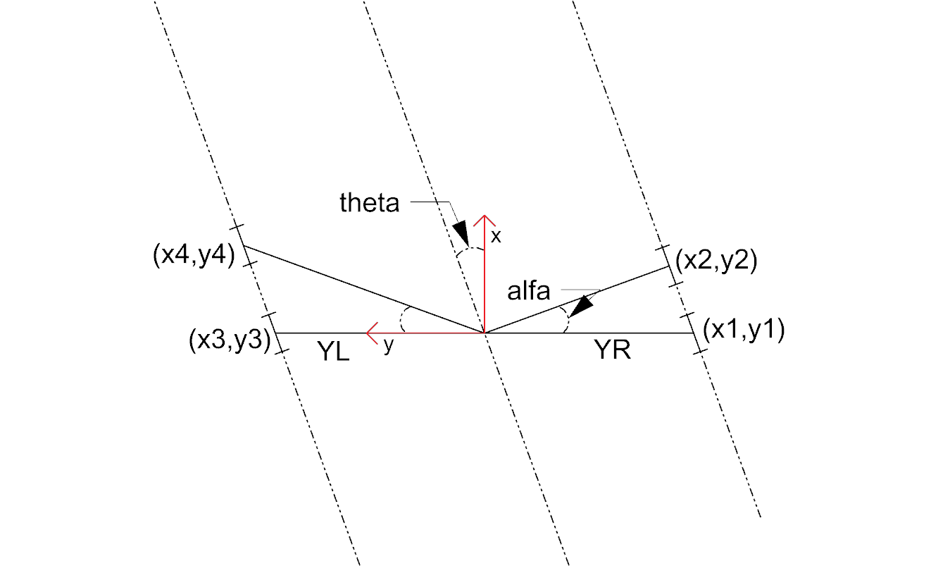
The laser distance node only uses a few laser points to determine the distance to the walls. In the figure below is shown how the distance is determined.

A couple of points direct next to PICO and in front of PICO are averaged and used for the distance calculations. The drawback of this approach is that only within a small region the walls are detected. Another drawback of this approach is that when the range of laserpoints that are averaged are not on a wall the distance and angle cannot be determined. because of these drawbacks is chosen to determine the distance to the walls based on lines.

Line distance

The calculation of the distance based on lines has several advantages in comparison to the laser distance.

• When the lines are used to determine the distance to the walls all the laser points are used instead of a small region of the laser points.
• When PICO is not between walls it is still posible to calculate a distance to the walls based on lines in front of PICO.

how the distance to the lines is calculated and implemented is described in the next part "implementation".

implementation

The input for this node are multiple points and every set of two points (x1,y1 and x2,y2) describe a line. To get the calculation of the distance to that line right the first step is to check what the orientation of the line is. We want to determine wheter the first point or the second point from the line closest to PICO. This is done very easy with the next piece of code:

       x1 = markers.points[i].x;
       y1 = markers.points[i].y;
       x2 = markers.points[i+1].x;
       y2 = markers.points[i+1].y;

       if (xx1>xx2){
           x1 = markers.points[i+1].x;
           y1 = markers.points[i+1].y;
           x2 = markers.points[i].x;
           y2 = markers.points[i].y;
       }

So in this situation the first point (x1,y1) is always in x-direction closest to PICO.

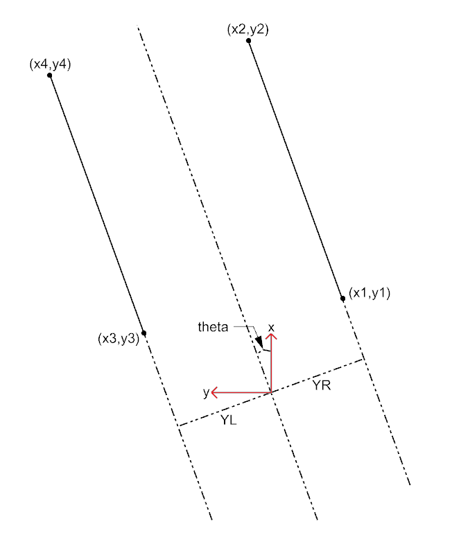
For every line the angle theta can be calculated with the next fomula:

[math]\displaystyle{ \theta = atan((y2-y1)/(x2-x1)) }[/math]

The position perpendicular to the line/wall is calculated with the next formula:

[math]\displaystyle{ Y = y2 - ((y2-y1)/(x2/x1))*x2*cos(\theta_1) }[/math]

This formula extends the line till next to PICO, so a line that is in front of PICO also results in a value for Y (left or right) as if the line is next to PICO. This is very usefull when PICO has turned and is not between the walls yet. The definitions of the distances are visualized in the figure below. Note that in the figure only the angle with respect to the centerline of the coridor is given but the distance node will give the angle to the left and right wall separated.

The two formulas described above are calculated for every line. Based on the values resulting from those formulas the lines are filtered. the next filtering criteria are used:

• The absolute value of the angle theta must be smaller than 0.785 rad (45 degrees):

this returns only the lines that are "vertical" (+ or - 45 degrees) for PICO.

• When Y > 0 a line is left from PICO.
• When Y < 0 a line is right from PICO.

After these filtering steps is it still possible that multiple lines are detected to the left or the right of PICO. So the next criteria was added:

• The line with the smallest Y value is used for the distance to the walls.

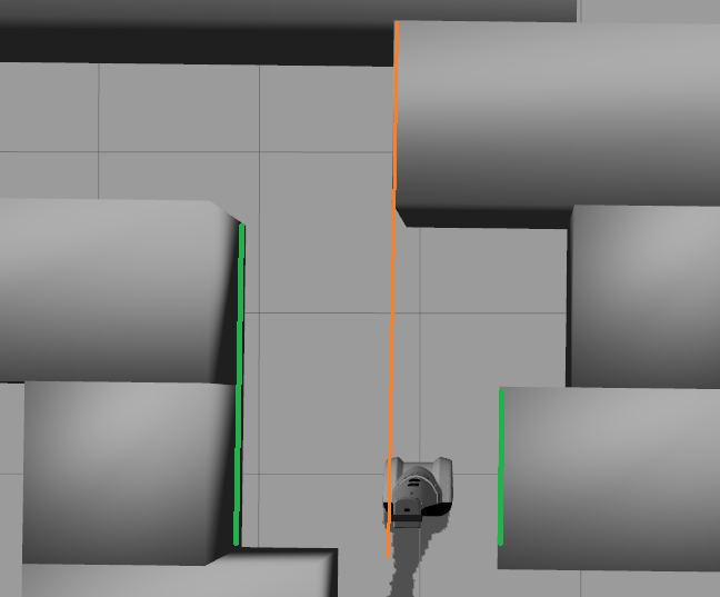
One critical situation when this approach might fail is shown in the Figure below. In that situation the wall in front of PICO (orange line) has the smallest Y value, so the distance to the orange line would give Y_left. But because PICO has only a few laser points on that wall it is not detected as a line so it wont give a problem and the distance relative to the two green lines will be returned.

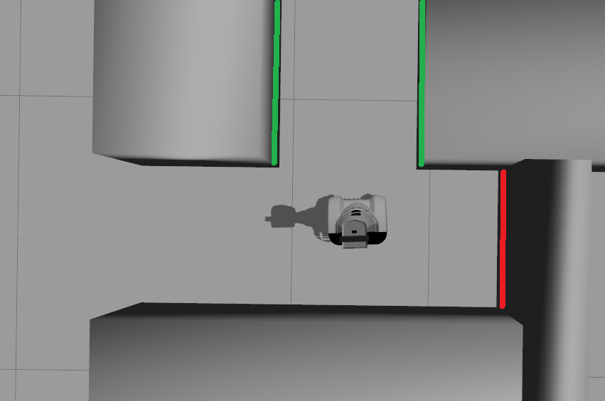
Another approach that was tested was to do the last filtering step based on the line with the x coordinate closest to PICO, so most of the time that is the line direct next to PICO. This resulted in problems when PICO turned towards a opening and a dead-end was left or right from PICO as shown in the figure below. PICO would then calculate the distance to the left wall of the opening and the right wall of the dead-end (red line).

Conclusion & recommendations

The calculation of the distance to the walls based on lines turned out te be very robust. This is aslo because the detected lines are very robust.

The only improvement that could be made in this part is the filtering of the lines. The last filtering step, the line with the Y coordinate closest to PICO, is a choice that we made and the control is adapted to this decision. For the control might not always optimal to know the distance to the line with the Y-coordinate closest to PICO though for the maze competition this was sufficient.

Odometry

Goal

The odometry block transforms the Quaternion odometry data to roll pitch and yaw angles.

Considerations

For the transformation the header file tf/transform_datatypes.h is included. No other options where found for this transformation.

Implementation

With use of the transformation the odometry data is transformed to roll, pitch and yaw angles. For PICO only the yaw angle is relevant, for that reason only the yaw data is published.

Conclusion & Recommendation

The odometry block is a very simple node. It publishes the yaw data which is used by the state machine to determine if PICO is turned.

Arrow detection

Goal

The goal for the arrow detection block is to detect arrows in the corridor by using the asus xtion camera mounted on PICO. Because of the strategy used mainly the to the left pointing arrow should be recognized to override the right wall folower strategy, however both directions are implemented.

Considerations

Three different approaches/methods are considered to achieve this goal:

• Template matching: Template matching is a technique which tries to find a reference image in the current 'video-image'. The technique slides the smaller reference image over the current image, and at every location, a metric is calculated which represents how “good” or “bad” the match at that location is (or how similar the patch is to that particular area of the source image). This is implemented using the openCV function matchTemplate, which results in a matrix with 'correlation' values from which a conclusion can be drawn where the template is matched best in the current image.

During testing of this technique it was found out that only one 'reference' of a certain size is used to compare to the image, in our case with our dynamical changing 'size' of our to be detected arrow we are only detecting the arrow correctly if the size of the camera image of the error is exactly the size of the reference arrow. Therefore to make this method work in our case we need a lot of arrow-reference images of different sizes, which is not suitable.

• Feature detection: Another approach is to use algorithms which detect characteristic 'features' in both the reference and camera image and attempt to match these. Because these features are generally not scale or rotation dependent, this method does not run into the same problems as described for template matching. Therefore, this approach was investigated in the following way:
  • The OpenCV library contains several algorithms for feature detection and matching. In general, some steps are followed to match a reference to an image:
    • Detect features or 'keypoints'. For this several algorithms are available, notably the SIFT and SURF algorithms. Generally, these algorithms detect corners in images on various scales, which after some filtering results in detected points of interest or features.
    • From the detected features, descriptors are calculated, which are vectors describing the features.
    • The features of the reference image are matched to the features of the camera image by use if a nearest-neighbor search algorithm, i.e. the FLANN algorithm. This results in a vector of points in the reference image and a vector of the matched respective points in the camera image. If many such points exist, the reference image can be said to be detected.
    • Finally, using the coordinates of the points in both images, a transformation or homography from the plane of the reference image to that of the camera image can be inferred. This transformation allows tells us how the orientation has changed between the reference image and the image seen by the camera.
  • Implementation of the previously described steps resulted in detection of the arrow in a sample camera image. However, it was found that the orientation of the arrow could not accurately be determined by means of the algorithms in the OpenCV library. Due to the line symmetry of the reference arrow, a rotation-independent detector would match equally many points from the 'top' of the arrow to both the top and the bottom of the arrow in the camera image, because the 'bottom' in the camera image can just as well be the top of the arrow when it is flipped horizontally. Therefore, the detector could not determine the orientation of the arrow, even if the full orientation is not of interest in this application.
  • One solution to the above problem could be to compare the vectors between the matched points in both images. Because it is only of interest whether the arrow is facing left or right, a simple algorithm could be defined which determines if many points which were located 'left' in the reference image are now located 'right', and vice versa. If this is the case, the orientation of the image has been reversed, allowing us to determine which way the arrow is pointing. However, this approach is probably quite laborious and a different method of detecting the arrow was found to also be suitable, which is why the solution described above was not pursued.

• Edge detection: By using the edge detection method, a arrow is recognized by analyzing the 'edges' of a red object within the camera image. This method is chosen because the implementation was proven to be simple and the conclusions to be drawn where correct and effective.

Implementation

Several steps are performed to recognize the edges of a red object within the camera image. Using those lines an eventual arrow can be detected. The steps are as follows:

• • Receive the rgb camera image.
  • Convert the rgb camera image to a hsv image.
  • This hsv image is converted to a binary image, red pixels are converted to white and all the other pixels are converted to black. A guided user interface (GUI) is implemented with slider bars to enable an easy selection of 'red' hsv values so that easy changes can been made during video playback.
  • Using a floodfill algorithm the 'red' area is smoothened out, (8 connectivity is used)
  • Edge detection is applied, as an edge is a 'jump' in intensity it can be recognized, this is done using a canny edge detection algorithm.
  • By using a hough transform lines are fitted through the detected edges.
  • CombineLines function is used to 'neaten' the lines which are coming out of the hough transform, documentation is found at the 'line detection' section because exactly the same code is used. By using CombineLines the performance of this method increased with a factor 2.5!
  • By recognizing the slanted lines (of about 30 degrees) the arrow head can be recognized. And the direction of the arrow can be derived.

To ensure robustness the arrow needs to be detected at least 2 times within 10 adjacent frames to be assumed valid and to trigger the 'arrow-detected' event. When within the 10 frames a false-positive is detected the counter of the amount of arrows (left or right) detected is reset to 0.

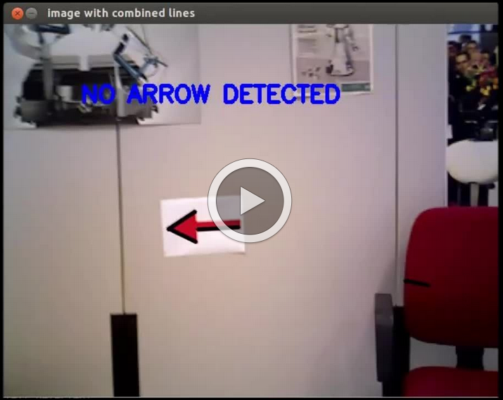
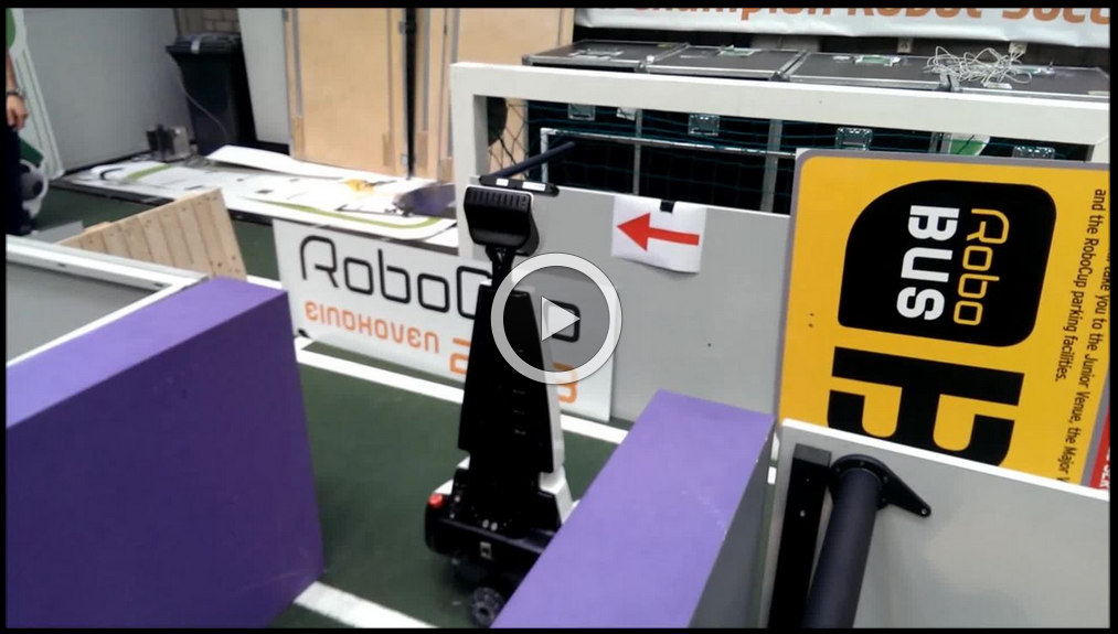
The result obtained is shown in the following videos, the left video showing an example of the edge detection (we use a right wall follower), and the right video a successful detection of an arrow by PICO within the maze:

Edge detection	PICO arrow in maze

Conclusion & Recommendation

After trying different techniques it was found that the edge detection approach was the most succesfull approach. It was found difficult at first to tune the right hsv - values for the red of the arrow under different lighting conditions, but by using the GUI it could be tuned eventually really easily. It can furthermore be recommended to find a way to stabilize the images so that an even better arrow recognition is possible. With the above described implementation PICO showed to recognize arrows robustly.

Finite State Machine

To successfully navigate a maze, PICO must make decisions based on the environment it perceives. Because of the multitude of situations it may encounter and the desire to accurately define its behavior in those different situations, the rules for making the correct decisions may quickly become complex and elaborate. One way two structure its decision making is by defining it as a Finite State Machine (FSM). In an FSM, a set of states is defined in which specific behavior is described. Events may be triggered by, for instance, changes in the environment, and may cause a transition to another state, with different behavior. By accurately specifying the states, transitions between states, and the behavior in each state, complex behavior can be described in a well-structured way.

Goal

The goal of this component is to provide a solid and easy to implement structure for high-level decision making of PICO. It must be possible to specify behavior in a modular way, such that testing, debugging and improving PICO's behavior is a straightforward procedure and PICO's decision logic can always easily de observed.

Considerations

As described above, structuring high-level decision making in the form of an FSM provides a powerful solution, in which behavior is can easily be determined by considering the state PICO is in. Several FSM packages exist for ROS:

• SMACH, a feature-rich task-level architecture for coordinating and executing behavior. However, SMACH is only available as in Python, while the remainder of our code is written in c++. Although it is possible to combine Python and c++ on runtime, this was considered too complex in the time frame of the course, therefore SMACH was disregarded.
• Decision_making FSM, a lightweight FSM solution available in c++. While promising, this package was available only for ROS Hydro, a more recent distribution of ROS than used in this course. In addition, it uses the catkin build system, whereas the older rosbuild system is used for this course. Therefore, this package too could not be used.

Because no off-the-shelf package for building an FSM was available, but the FSM logic was considered the most suitable to the current objectives, a custom FSM system was built. This system must meet the following requirements:

• Provide essential FSM functionality: configure and execute an FSM with event-based transitions between states
• Abstract 'operational' logic so that it can be applied without having to consider the inner workings.
• Provide an easy to use and logical interface to configure and run the FSM.

Implementation

To ensure clean code and a well-structured system, the custom FSM was written in OOP as its own class. Inner logic is defined through private methods, with only a constructor and relevant public methods for manipulating and executing the FSM.

Functioning

States and events constituting a transition between states are internally described as integers and can be defined after instantiation of the FSM. Transitions can be registered by supplying the begin state, event and target state. After defining all states, transitions and an initial state, sensors can send events to the FSM which may trigger a transition, if such a transition is available from the current state. Because ROS uses a polling system with a definable update frequency, multiple events can be received at once. These are therefore collected in a vector, which then contains all available events at that time instance. By executing the FSM, the system runs through all available events and checks if that event can trigger a transition from the current state. If this is the case, the current state is updated to the transitioned state. To ensure unambiguous behavior, care must be taken that multiple events that can each trigger a transition do not occur at once; otherwise, the FSM can result in undesired behavior. This can be prevented by updating and executing the FSM at a high enough frequency and by proper definition of the states and transitions.

To further facilitate configuration of the FSM, special 'panic' transitions can be registered. These transitions are made available from all states and can be used for, for instance, detecting collisions and going into a safe mode. Use of panic transitions thus eliminates the need to register this transition for each state, which could easily lead to errors when new states are introduced.

To ensure all nodes use the same integers to describe an event or state, these were defined as constants in Event and State messages, which could then be accessed by any script which includes them. This way, states and events could be referenced to in human-readable form, further improving readability and preventing errors.

Interface

The following methods are used to configure and run the FSM:

• fsm(int state_init) Instantiates the FSM object and stores the initial state.
• tr(int state_from, int event, int state_to) Registers a transition from a state to another state by an event. Transitions are stored in a vector of structs containing the three integers.
• panic(int event, int state_to) Registers a special transition which is available from any state.
• clearEvents() Clears the list of available events.
• makeAvailable(int event) Adds an event to the list of available events for the next time the FSM is run.
• int runOnce() Runs the FSM, making a transition to a new state if an available event was found in the list. Iterates over all transitions, calling the private method tryTransition() (see below). Returns the new state.

Inner logic

• bool isAvailable(int candidate) Searches the list of available events for the given candidate event, returning true if it is found or false otherwise.
• tryTransition(int event, int candidate_state) Attempts to make the given transition from the current state. Checks if the transition can be made by running isAvailable(), updates the current state if true is returned.

Implementation in ROS

In this implementation, decision making is executed from the behavior control node, which instantiates and configures the FSM. Events can be published from any node to a dedicated topic /pico/events, which is listened to by the behavior control node. The received events are periodically pushed to the FSM system, which is the run using the runOnce() method. The received, possibly changed state is then published on the /pico/state topic to be used by any other node which requires it. Furthermore, now the current state has been decided, the correct behavior for PICO is executed. This low-level behavior is in this implementation defined in a separate class, containing functions for each of the behaviors PICO can perform, and executed through a public perform() method. More about this can be read in the Behavior control section.

Conclusion & Recommendations

The developed FSM system provides an easy structure to define high-level decision making for PICO, requiring little configuration and abstracting the heavy lifting of its inner workings. Events can be triggered from any process and the resulting state can be used by other processes. The system allows for simple developing, tuning, altering and debugging of the behavior. The solution is lightweight and adds little overhead to the program. It can also be used in different implementations, not relying on a particular process it is run from or logic it is used in.

The system could be further improved to include execution of the desired behavior directly by the FSM, by registering a function call to each state. This way, configuration of the FSM can fully determine the behavior of PICO, making the process of developing behavior even more transparent. An improvement in the implementation could be made, in which multiple FSM instances can be used to define a hierarchical state machine. A state could contain an FSM of its own, allowing consecutive or other more complex behavior to be performed, before transitioning to a new 'master state'. Due to the relatively simple behavior in this course, this was not implemented.

Situation Recognition

Goal

• Provide relevant parameters about the situation PICO is in for high-level decision-making.
• List of interesting detections: non-dead exit L/R, wall L/R, front wall approaching, dead end.

Considerations

• Full situation doesn’t need to be determined; send only relevant data (mostly events for FSM).
• Laser data can be used for some parts (exits, corridor), but difficult for more complex situations (dead end, ‘dead exit’).
• Based on lines still complex (meaning of different line segments), but ‘fewer DOF’.
• Finite brackets method -> difficult with angles, not really leveraging lines.

Implementation

• Only when ‘relatively straight’; group lines left/right/front/back.
• Scan sides for exit, check for non-dead, determine if wall to side for end-of-turn, determine exit width.
• Scan front for wall ahead, dead end or only-exit-left.
• Dead end and exit width determined only once per exit, use of counter for robustness.
• Collision/release.
• Left/right using same functions, changing ‘direction_sign’ parameter

Conclusion & Recommendations

• All interesting situations robustly determined (in all maze simulations and in testing).
• Limitation: implementation for local (event-based) planning only, if ‘global’ planning desired, can be rewritten to output relevant data.

Behavior control

The ultimate objective of the software architecture is to steer PICO in the desired direction. Using a State Machine to determine the action PICO should take, the information supplied by each component can be used for robust control and high performance.

Goal

The goal of the behavior control component is to use the information received from other components to provide input to Drive component for desired behavior.

Considerations

High-level decision making is performed using an FSM instance. In each state, some behavior function can be defined. Therefore, in these low-level behavior control functions, we do not need to be concerned with when some behavior is performed, but only how that behavior can be characterized. Because of the holonomic platform with two translational and one rotational DOF and the restriction of driving between walls, only a limited set of behaviors needs to be defined. By separating the behavior control component into high-level decision making and low-level behavior functions, behavior shared by different states does not need to be defined multiple times, reducing code complexity and ensuring well-defined behavior in each situation.

Implementation

• Describe how FSM triggers some behavior function
• Describe behavior functions (drive FW, rotate in place, ‘smooth cornering’)
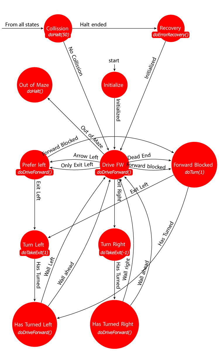
• FSM decision tree with states, transitions, and behavior in states.

Robustness

Safety

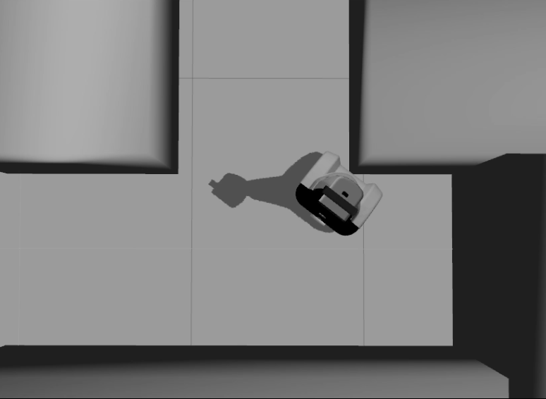
To prevent PICO from hitting the wall some extra safety measures were implemented. The first measure was to let PICO stop when it is to close to a wall or other object. This is done by scanning over all the laserpoints and when a point is between 30 and 15 cm of Pico it will stop driving. The 15 cm is there because the first and the last couple of points wil see PICO itself and that distance is smaller than 15 cm. So when a laser point is within 15cm it is probebly PICO's own body.

From the beginning this was implemented to prevent PICO from hitting a wall but there was nog recovery if PICO got into "collision".

From every state the transition to the collision state is posible but there was no transition from that state to another state. If PICO goes in the collision state because of for instance someone walks in front of PICO, it dont has to recover. In that situation PICO only has to stop driving for a while and continue driving when the "danger" is gone. To implement that the previous state (before the collision) must be known and a transition from the collision state to every other state must be posible. So when the event "danger" is not longer triggered PICO goes back to the previous state and continues its way.

If PICO is in the collision state for a cetrain time than PICO will be posibly close to a wall or other object and it has to "recover". To recover PICO it drives backward for about 25 cm and while it is driving backwards it will position to the detected walls. If only one wall is detected it will allign at a certain distance from that wall but if two walls are detected PICO will align in the middle of that corridor. After aligning PICO will continue in the state "drive forward". In some cases it will be posible that PICO drives trough the maze in the wrong direction (after recovering), and will go back to where it started. This is always better than when it is just standing still in the maze and someone had to find it somewhere in the maze to reset it.

An example of the implemented safety is shown in the movie below:

Safety

State Machine

Conclusion & Recommendations

• All important behaviors implemented.
• Improvements: ‘fully’ smooth cornering

Drive

Goal

The drive node sends velocity commands to PICO based on information from the line distance and state machine. The line distance gives information about PICO's relative horizontal and angular position with respect to the walls in front. The state machine gives, if applicable in the state, an angular speed and a speed in forward direction. The goal of the block is to determine in which case PICO needs to use the the state machine information, line distance information or both.

Considerations

For the drive node a custom C++ code is written. The main function of the block is to determine in which case PICO needs to use the the state machine information, line distance information or both.

The state machine gives straight forward velocity information [math]\displaystyle{ (\dot{x} }[/math] and [math]\displaystyle{ \dot{\theta}_{turning}) }[/math] which can be used immediately as velocity command.

The line distance node provides the left and right horizontal distance to a wall [math]\displaystyle{ (Y_L }[/math] and [math]\displaystyle{ Y_R) }[/math]. Furthermore the relative angle left and right of PICO is provided [math]\displaystyle{ (\theta_L }[/math] and [math]\displaystyle{ \theta_R) }[/math]. This information needs to be interpreted to position and orientate PICO with respect to the walls. This control is called position control.

The position control of PICO cannot always be used. For example, PICO needs position control when it is driving in a corridor. Though when PICO is turning for an exit the position control cannot be used because this will give strange behavior. Furthermore when PICO needs to use position control there are situations where only one wall is on the left or right side. Also it is possible that no lines are detected in a close region from PICO. This needs to be interpreted robustly for a good behavior of PICO through the maze.

Implementation

The determination if PICO needs to use position control is implemented in a simple way. If the state machine sends an angular velocity [math]\displaystyle{ (\dot{\theta}_{turning}) }[/math] which is not zero no position control will be applied. In that case [math]\displaystyle{ \dot{x} }[/math] and [math]\displaystyle{ \dot{\theta}_{turning} }[/math] are send as velocity command to PICO. In all other cases position control will be used. In those cases the velocity [math]\displaystyle{ \dot{x} }[/math] from the state machine and the output of the position controller will be send [math]\displaystyle{ (\dot{y} }[/math] and [math]\displaystyle{ \dot{\theta}_{orientation}) }[/math].

For the position controller different determinations of [math]\displaystyle{ (\dot{y} }[/math] and [math]\displaystyle{ \dot{\theta}_{orientation}) }[/math] are possible depending on the input data. The basic position control is a simple proportional controller. In the general case (when two walls are detected) the difference between the left and right horizontal position is determined. This value is multiplied with a gain (0.6) and send as a velocity command to PICO.

[math]\displaystyle{ \dot{y}=(Y_R+Y_L)\cdot y_{gain} }[/math]

For the angle the average between the left and right angle is taken and also multiplied with a gain (0.4).

[math]\displaystyle{ \dot{\theta}_{orientation} = ((\theta_R+\theta_L)/2)*\theta_{gain} }[/math]

This approach gave good results during simulations and testing so no additional control blocks (for example PD controller) are used.

The other options for position control are:

• Wall detected on either left or right side: PICO will drive 0.5m from the detected wall and orientate on this wall.
• No walls detected: no position control will be applied.

Conclusions and Recommendations

The drive node is a simple node that sends the velocity commands to PICO. Simulations and experiments have shown that PICO is able to drive robustly through every situation for the maze. The robustness is the effect of the simple approach used in this node.

Improvements to this node can be made by adding a derivative part to the position controller, though as already stated it functions very robust with the current implementation.

Software overview

The table below gives a summary of all the software components described in detail above.

Node	Subscibes topic:	Input	Publishes on topic:	Output	Description
Line detection	/pico/laser	Laser scan data	/pico/lines	Array of detected lines. Each line consists out of a start and an end point (x1,y1),(x2,y2)	Transformation of raw data to lines with use of the Hough-transform. Each element of lines is a line which exists out of two points with a x- y and z-coordinate in the Cartesian coordinate system with Pico being the center e.g. (0,0). The x- and y-axis are meters and the x-axis is the front/back of Pico while the y-axis is left/right.
Arrow detection	/pico/camera	Camera images	/pico/vision	Arrow detected to the left of the right	Detection of arrows pointing to left or right.
Odometry	/pico/odom	Quaternion matrix	/pico/yaw	float with yaw angle	Transform Quaternion in roll, pitch and yaw angles. Only yaw angle is sent because roll and pitch are zero.
Distance	/pico/line_detection	Line coordinates	/pico/dist	(y_left, y_right, x, theta_left, theta_right) also known as the 'relative position'	Determine distance to wall to left, right and front wall. Also determines angle left and right with respect to the walls.
Situation	/pico/line_detection /pico/laser /pico/vision	Line data, vision interpretation and possibly laser data.	/pico/situation	The situation where pico is in. For example corridor to the right, T-junction, etc.	Situation parameters.
State generator	/pico/situation /pico/yaw	Situation and yaw angle of Pico.	/pico/state	dx,dy, dtheta	Based on the situation Pico needs to go through different states and continue to drive. Every state defines an action that Pico needs to do.
Drive	/pico/state /pico/dist	(y_left, y_right, dy, x, dx, theta_left, theta_right,dtheta)	/pico/cmd_vel	Pico moving	Move pico in the desired direction

Corridor competition

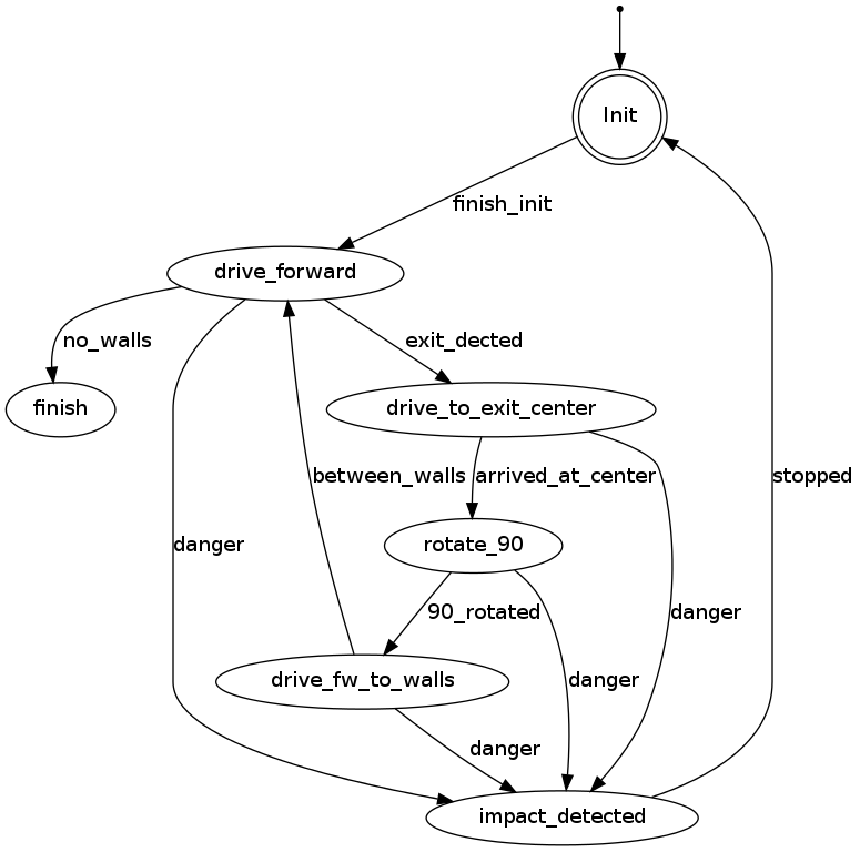
For the corridor challenge a straight forward approach is used which requires minimal software effort to exit the corridor succesfully. As a result only the nodes laser and encoders are used for driving.

Approach

For PICO the following approach is used to solve the corridor challenge.

• Initialize PICO
• Drive forward with use of feedback control
  • A fixed speed is used, i.e., [math]\displaystyle{ v }[/math]
  • Safety is included by defining the distance from PICO to the wall (determined with use of the laser data). PICO will stop if the distance becomes [math]\displaystyle{ \lt 0.1 }[/math]m
  • The distance between the left and right wall is calculated with use of the laser data. With this input PICO will stay in the middle of the corridor.
  • The angle of pico relative to the walls is used to keep PICO oriented in the same direction as the walls.

• If an exit is detected, feedforward control is used
  • PICO drives for [math]\displaystyle{ T_e }[/math] [s] to ensure that it is orientated in the middle of the detected exit.
  • After [math]\displaystyle{ T_e }[/math] [s] PICO rotates +/-90 degrees using the odometry
    • +/- depends on which side the exit is detected
• When PICO has turned drive forward is again enabled to drive to the detected exit
  • Safety is included by defining the distance from PICO to the wall (determined with use of the laser data). PICO will stop if the distance becomes [math]\displaystyle{ \lt 0.1 }[/math]m
• PICO detects the finish (out of corridor) when no walls are detected
  
  

The states that are described above are visualized in the following figure:

Result

The corridor competition was a succes. PICO drove straight through the corridor and when the exit was detected it turned 90 degrees and drove out of the corridor. Two things that were observed(also during testing)

• Turning 90 degrees on the odometry is not always the same for every situation.
• Gaps within the corridor are influencing PICOs behavior
  

The key to our victory (in the fast group) was that we used simple and straightforward approach to exit the corridor. During the competition some confusion was present about the maximum speed of PICO (we used a speed of 0.4m/s, because in the lecture were it was mentioned that the velocity of PICO was limited to 0.2m/s we were busy testing). Therefore the jury decided to announce two winners (slow and fast winners).

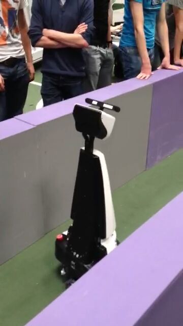
The result of the corridor competition is shown in the movie below.

Corridor competition

Problems/Bottlenecks

• The odometry data is not always reliable
  • As a result of the varying friction force, between the wheels and the ground
  • Must be taken into account to increase robustness
• The laser data is not robust when gaps are present within the corridor
  • Will be improved when using line data instead of laser data

Maze competition

Result

The maze competition was a succes. PICO was able to detect dead-ends that were present in the beginning of the maze. In the maze also two arrows were present which were succesfully detected by PICO. In the final corridor the robustness of PICO was checked (with succes) due to the fact that the width of the corridor changed.

Nevertheless, we finished on the 3th place (the difference between the first and third place was ~2 second). The group that won were able to drive around the corners more faster. The minor difference between the first and the third place indicates that we performed an excellent job!

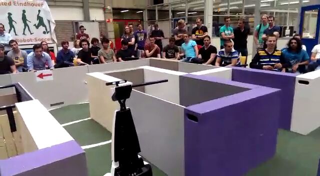
The result of the maze competition is shown in the movie below.

Maze competition

Conclusions and Recommendations

Conclusions

We were able to construct a fast maze/corridor solving PICO, which has a

• Modular design
• Plug&play state machine which makes it easy to add additional states
  • Describes new behavior of PICO
• Robust design (as shown in the movie below)
  • Able to solve a dynamic maze
  • Able to detect different objects that block its path
    • For instance humans
  • Gaps within the corridor does not influence PICOs behavior
  • Red arrows are detected in different environments (different light brightness)

Recommendations

Possible extensions for a faster maze solving PICO are:

• Cornering can be optimized
  • Start with broaching just before the corner
• Implement Tremaux's algorithm
  • The Tremaux's Algorithm solves a maze by marking how many times a passage has been passed.
  • With this algorithm PICO will also be able to solve a more complex maze

Appendix

Appendix A. Planning

Week 1 (2014-04-25 - 2014-05-02)

• Installing Ubuntu 12.04
• Installing ROS
• Following tutorials on C++ and ROS.
• Setup SVN
• Plan a strategy for the corridor challenge

Week 2 (2014-05-03 - 2014-05-09)

• Finishing tutorials
• Interpret laser sensor
• Positioning of PICO

Week 3 (2014-05-10 - 2014-05-16)

• Starting on software components
• Writing dedicated corridor challenge software
• Divided different blocks
  • Line detection - Sander
  • Position (relative distance) - Richard
  • Drive - Marc
  • Situation - Wouter
  • State generator - Joep
• File:Presentatie week 3.pdf

Week 4 (2014-05-17 - 2014-05-25)

• Finalize software structure maze competition
• Start writing software for maze competition
• File:Presentatie week 4.pdf

Week 5 (2014-05-26 - 2014-06-01)

• Start with arrow detection
• Additional tasks
  • Arrow detection - Wouter
  • Update wiki - Sander
  • Increase robustness line detection - Joep
  • Position (relative distance) - Richard
  • Link the different nodes - Marc

Week 6 (2014-06-02 - 2014-06-08)

• Make arrow detection more robust
• Implement line detection
• Determine bottlenecks for maze competition
• Make system more robust

Week 7 (2014-06-09 - 2014-06-15)

• Implement Arrow detection
• Start with more elaborate situation recognition for dead end recognition
• Test system

Week 8 (2014-06-16 - 2014-06-22)

• Improve robustness
• Finish dead end recognition

Week 9 (2014-06-16 - 2014-06-22)

• Improve robustness of system for maze competiotion

Appendix B. Meetings

Weekly meetings are planned during the course. Every Wednesday a standard meeting is planned to discuss progress with the group and with the tutor. Presentations from these weekly meetings can be found with the presentation links below. Important meeting decisions can be found with use of the meeting liks below. Next to the standard weekly meetings evening meetings are planned to work as a group on the software design. For some meetings the minutes can be shown by clicking on the hyperlinks below.

1. Meeting - 2014-05-02
2. Meeting - 2014-05-12
3. Meeting - 2014-05-14
4. Meeting - 2014-05-15
5. Meeting - 2014-05-16
6. Meeting - 2014-05-21
7. Meeting - 2014-05-23
8. Meeting - 2014-05-27
9. Meeting - 2014-05-28
10. Meeting - 2014-06-02
11. Meeting - 2014-06-04
12. Meeting - 2014-06-05
13. Meeting - 2014-06-06
14. Meeting - 2014-06-11
15. Meeting - 2014-06-13
16. Meeting - 2014-06-18
17. Meeting - 2014-06-20
18. Meeting - 2014-06-25
19. Meeting - 2014-06-27
20. File:Presentatie week 3.pdf
21. File:Presentation week 4.pdf
22. File:EmbeddedMotionControl01 wiki.pdf

Appendix C. Group Info

Name:	Student id:	Email:
Groupmembers (email all)
Sander Hoen	0609581	s.j.l.hoen@student.tue.nl
Marc Meijs	0761519	m.j.meijs@student.tue.nl
Wouter van Buul	0675642	w.b.v.buul@student.tue.nl
Richard Treuren	0714998	h.a.treuren@student.tue.nl
Joep van Putten	0588616	b.j.c.v.putten@student.tue.nl
Tutor
Sjoerd van den Dries	n/a	s.v.d.dries@tue.nl

Appendix D. Videos

Simulation

Corridor challenge	Line detection	Maze

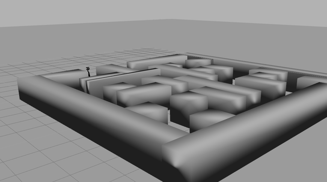Real-time

Corridor challenge	Maze
Edge detection	PICO arrow in maze
Robustness	Safety

Appendic E. PICO messages

The different nodes are communicating with each other by sending Messages. Each nodes sends a set of messages with use of a publisher. The Message that are sends between the nodes are defined in this section.

Lines

The line message includes two points, p1=(x1,y1) and p2=(x2,y2), which are defined by the geometry messages package. A point consists of (x,y,z) coordinate. For points p1 and p2 the z-coordinate is set to zero.

Points p1 and p2 are connected to represent a line each line is stored in array:

  line[] lines

Duplicate lines are merged to one line. The detected lines are visualized as a Marker in rviz, by using the visualization_msgs package.

Vision

The vision message contains two booleans for if it either detects an arrow pointing to the left, or a arrow pointing to the right.

   bool arrow_left
   bool arrow_right

Distance

The distance message contains the following floats

   float32 YR
   float32 YL
   float32 THR
   float32 THL
   float32 X 

Determining the distances from pico to the detected walls.

Situation

Basically, there are eight main situations, these are shown in the figure below. If PICO does not detect any corner points, then it is located in a corridor. In this case the robot can go straight on. If PICO detects any corner points, then it might need to turn. Whether it needs to turn, depends on the situation. The different type of situations are

   Situation T-junction exit left right
   Situation T-junction exit front right
   Situation T-junction exit front left
   Situation Corridor
   Situation Corridor right
   Situation Corridor left
   Situation Intersection
   Situation Dead end

State generator

A Finite State Machine (FSM) is used to structure the decision making of pico. In an FSM, a set of states is defined in which specific behavior is described. The different state are denoted below

   State Initialize
   State Drive Forward
   State Arrow Left
   State Dead End
   State Turn Left
   State Turn Right
   State Dead End
   State Has Turned
   State Has Reversed

An overview of the different states and how they are connected will be illustrated in section Software components - State generator

Drive

The drive message sends commands to the drive node which actually sends the velocity commands to pico. The message contains two float32, one to specify the velocity forwards and one to represent the velocity by which Pico turns around his axis.

   float32 speed_angle
   float32 speed_linear