Embedded Motion Control 2014 Group 10

Members of group 10

Bas Houben	0651942
Marouschka Majoor	0660462
Eric de Mooij	0734166
Nico de Mooij	0716343

Planning

Week 1

• Introduction
• Install Ubuntu

Week 2

• Determine the course goals
• Brainstorm about the robot control architecture
• Start with the tutorials

Week 3

• Continue with the tutorials
• Install ROS/QT
• Finish robot control architecture
• Brainstorm about collision principle
• Brainstorm about navigation

Week 4

• Meet with the tutor
• Finish installation
• Finish tutorials
• Write collision detection
• Write corridor navigation
• Test the written code on Pico
• Corridor challenge (Recorded performance)

Week 5

• Meet with tutor
• Software structure designed
• Started working on the scripts

Week 6

• Meet with tutor
• Software structure design rejected and redesigned
• First target point/dijkstra based algorithm
• Pico experiment

Week 7

• Meet with tutor
• Target point changer added
• Artificial blind spots added to the algorithm
• Arrow detection algorithm designed
• Experiment

Week 8

• Prepare final presentation
• Final presentations
• Start/Finish detection added
• Double check for deadlock added
• First version of Arrow detection added
• Pico experiment

Week 9

• Meet with tutor
• Final version of Arrow detection added
• Arrow detection tested on multiple cases with different red patterns in it.
• Pico experiment
• Maze competition

Concepts

Robot program architecture

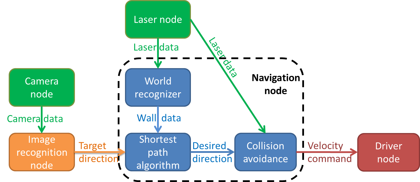
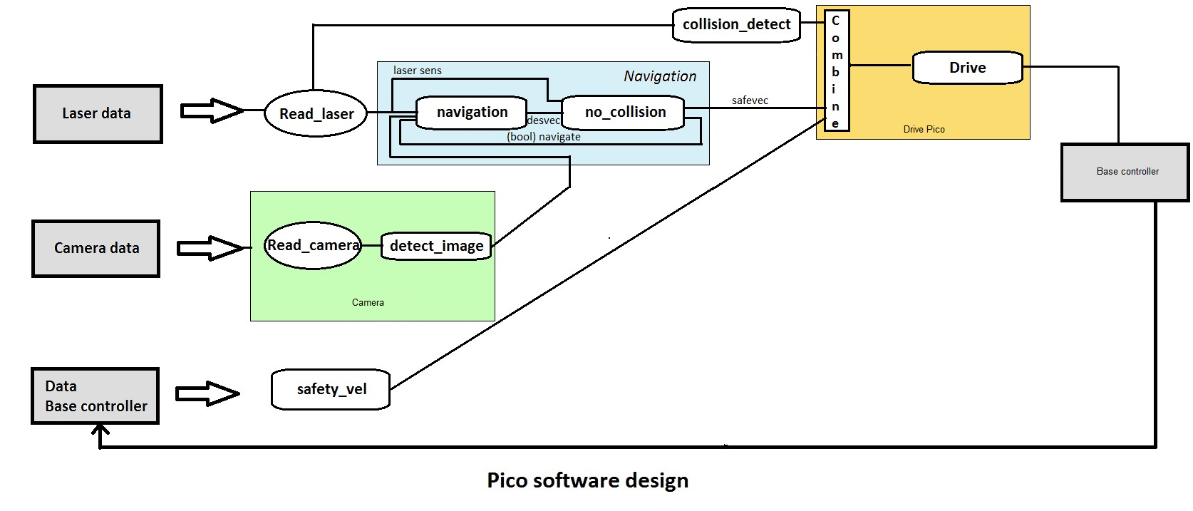
While the initial idea was to give every distinguishable function its own node, several main functions have been placed together in one node, because they have to communicate large matrices with each other. Besides the laser, camera and drive node's provided by the course, we added two additional ones: the image recognition node and the navigation node. The main functions and their interactions can be seen in the image below.

The program runs three consecutive main steps, listed below.

Determining strategy

In the first step, pico determines what strategy to apply, depending on whether an arrow is detected or not. The default strategy is to follow the wall to the right, executed by taking every right turn available. From now on, this method will be called the 'right hand rule'. When an arrow is detected in the distance, the strategy is changed to driving straight forward, towards the arrow. If the arrow is close enough to take the turn, the strategy is set to either the right hand rule or left hand rule, according to the direction of the arrow. When no arrow is detected, the strategy will return to the default right hand rule. This step involves the 'Camera node' and the 'Image recognition node', which will be explained in more detail later. The 'Camera node' sends camera data to the 'Image recognition node', which then searches for an arrow. The image recognition node provides a target direction for the second step, according to any arrows it might recognize.

Path finding

In the second step, the strategy determined by step one will be executed with the aid of Dijkstra's shortest path algorithm. This algorithm detects whether a turn is available, and whether it has a dead end or not. It then calculates an optimal path according to the turn options available. This step involves the 'Laser node' and the 'World recognizer" and 'Shortest path algorithm' functions of the 'navigation node'. These two functions will be explained in further detail later on. The 'Laser node' sends laser data to the 'World recognizer' function, which makes a map of the walls currently visible, and stores it in a matrix. The 'Shortest path algorithm' function uses this matrix to determine an optimal path. This optimal path is converted to a desired direction vector, which is used in the third step.

Collision avoidance

In the third step, the desired direction vector provided by the previous step is checked for collisions, and altered accordingly. This involves the 'Laser node' and the 'Collision avoidance' function of the 'Navigation node'. The 'Laser node' provides the 'Collision avoidance' function with laser data. This data is used to determine if any walls come within a certain safety range. When this occurs, the desired direction provided by the previous step is altered to avoid collisions. If no collisions are imminent, the desired direction is left unaltered. The possibly altered desired direction is transformed to a velocity command, which is then send to the 'Driver node'.

Robot program architecture

The idea of our architecture is to create different process layers. By splitting the incoming signals and combining them later, the tasks can be divided and the different processes can run in parallel. Layers are based on the available sensors as much as possible.

Wall detector

The wall detector determines whether the robot is close to a wall or not by determining the unblocked distances at its two sides. When either side is too close (within 30cm) it turns parallel to that side, taking a distance of 30cm from the wall.

Intersection detection for corridor

At the time of the corridor competition, the path planning algorithm was not yet completed. Instead, a simple intersection detection was implemented. The idea behind this concept is that Pico will look at the laserdata of a certain range.

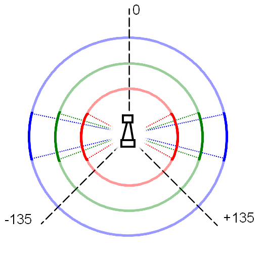
Pico will look left and right. If the laserdata returns that all the distances inside the range are higher than a certain value, a corridor might be present. In order to double check this, a second and third check are performed with more narrow angles and higher minimum values. This method is shown in the image below.

For Pico to recognize a corridor, it must be at least 60 cm wide. The three ranges that are checked are 0.5 m, 1.0 m and 1.5 m. This corresponds to ranges of 74, 35 and 23 degrees.

Once a corridor is detected, Pico will stop moving forward. He will then turn into the direction of the exit and drive out of the corridor. The collision avoidance system will once again make sure Pico does not hit any walls as he is driving out of the corridor.

Intersection determination

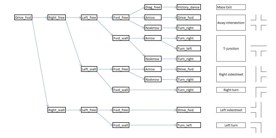
Depending on the results from the intersection detection part, Pico will determine which situation he is in. In the maze, these situations could be 4-way intersection, corners and T-junctions. The image below shows how each situation is determined depending on the presence of a wall or corridor in the forward, left or right detectors. At this point, arrows can not yet be detected, so that part of the protocol is skipped. Once arrow recognition is implemented, the arrows will be used to determine the correct corridor to take at T-junctions, or to move towards a T-junction at the end of a corridor, if an arrow is detected in the distance.

Moving through intersections and corners

Once Pico has detected a situation and determined if he want to turn, he will rotate + or - 90 degrees. After the rotation, Pico will drive forward a small distance to position himself fully into the next corridor and will look around once more.

Encountered problems

Corridor code

While programming the corridor code, few problems were encountered. Aside from several compilation errors, the simulations went without any problems. However, the experiments prior to the corridor competition did pose several difficulties. The rotational velocity in gazebo is limited at 0.5 rad/s, but the actual robot did not have such a limitation. Since the rotational velocity in the script was way higher than 0.5 rad/s, the collision detection was over-tuned, resulting in a saw-tooth like path. Additionally, the 90 degree turn was incorrect as well, due to the rotational velocity of over 0.5 rad/s. Both problems were solved by properly re-tuning the rotational velocity constant.

Dijkstra's algorithm

As is common with computations as complicated as Dijkstra's shortest path algorithm, several compilation errors were encountered in this part of the code. These were solved by standard compilation error solving techniques. Aside from these compilation errors, several functionality bugs had to be solved. The first bug was caused by improper matrix sizes, resulting in 'segmentation faults'. By expanding both the path storage and cost function matrices, these problems seemed to be solved. In certain cases, however, the segmentation faults continued to exist. This turned out to be caused by not programming the boundaries of the grid, and thus the storage matrix, in algorithm. By implementing these boundaries, several strange numbers in the grid matrix disappeared as well. The boundaries for the walls has been set at the 2nd layer, keeping the outer layer unoccupied. This allows the algorithm to go around walls that reach to the edge of the grid, preventing unnecessary deadlocks. After this change, the algorithm function properly. However, the desired results were not yet obtained. Pico could drive backwards that was shorter, and often turned back into the corridor he just left.

To let our pathing algorithm work as intended, we had to apply some modifications to Dijkstra's algorithm. First, we added the blind spot of pico, and modeled it as a solid wall. This solved the problem of driving backwards. However, pico could still turn back in corridors he had just left. Our first idea to prevent this, was adding a short term map memory. By letting walls remain in the algorithm for a few seconds after disappearing from pico's sight, we would have solved pico's tendency to turn back into corridors, while simultaneously preventing pico from displaying indecisive behavior at moments that walls disappear from the grid. However, short term wall memory turned out to be very hard to implement. With pico driving around and turning simultaneously, the position of old walls had to be corrected often and accurately. Because we did not know the exact position of the laser range finder relative to pico's rotational axis, we did not manage to apply the proper coordinate transformations to the wall. Furthermore, wall memory proved to be extremely susceptible to ghost points, whose harmful effects were amplified by the inflation of the walls in the grid. All these factors combined prompted us to look for alternative solutions.

Our next idea was to block of the old entrance with artificial blind spots. While relatively simple, this idea proved to be surprisingly effective. After some tuning of the blindspots shape, we solved both the indecisive behavior and pico's tendency to turn back into the corridor he just left.

Arrow Detection

To recognize or a given arrow is pointed to the left or to the right, and to let Pico react on this, several steps are followed while driving Pico.

Steps performed for all pictures:

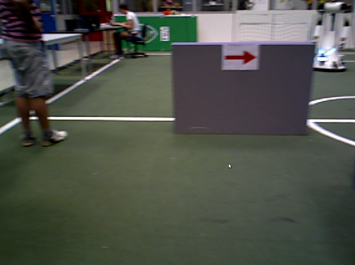
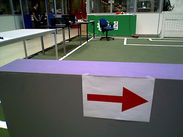
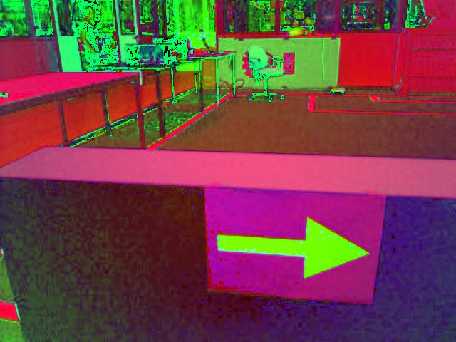
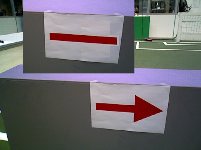
Step 1: The ROS image is converted to an Open CV image. Picture used as example:

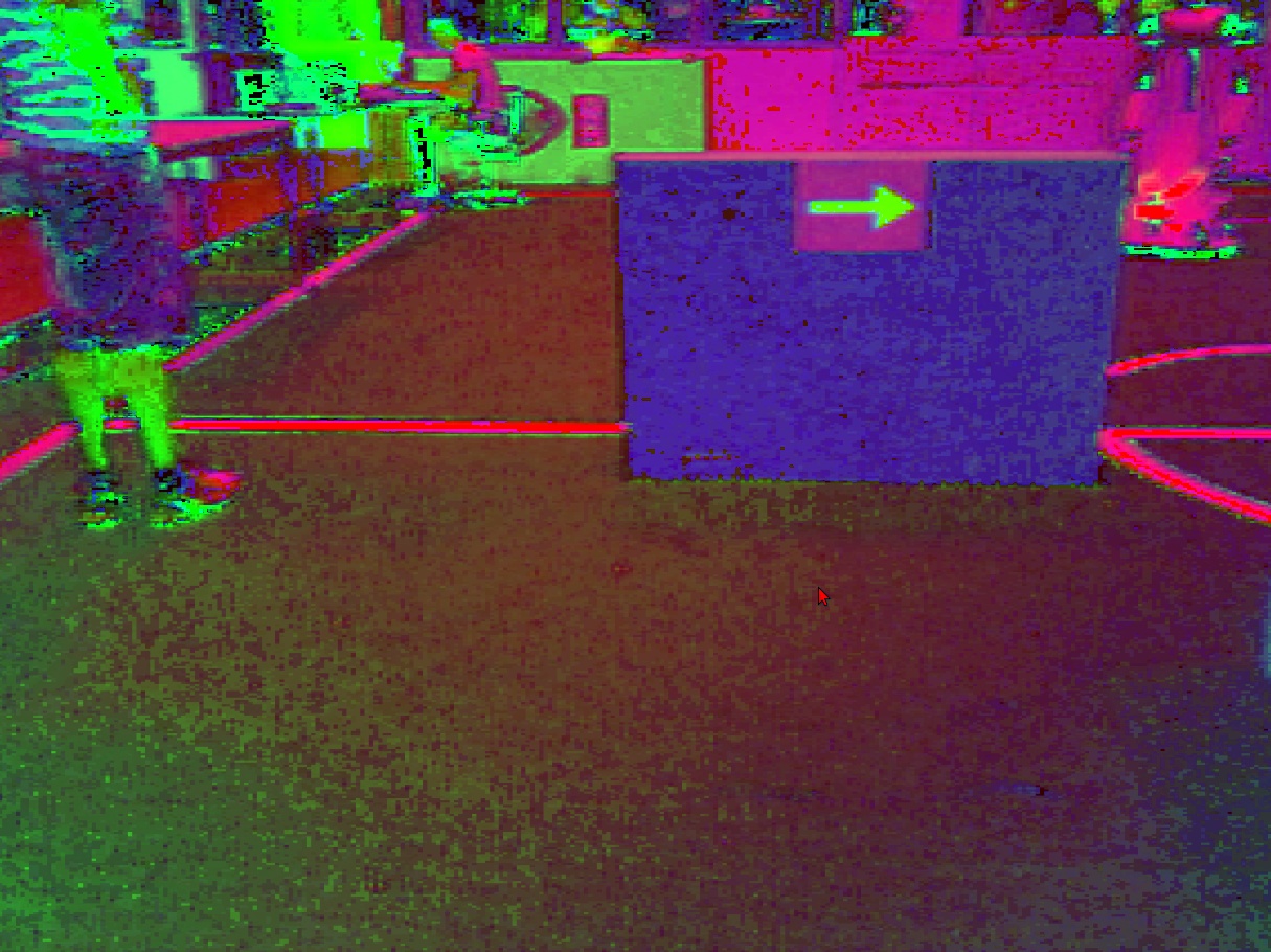
Step 2: There are different color spaces to describe pictures. In our case the RGB image is converted to an HSV image using the OpenCv function cvtColor and option CV_BGR2HSV. HSV is commonly used in computer based graphic design. Converting RGB to HSV and vice versa is unambiguous. This results in the following picture:

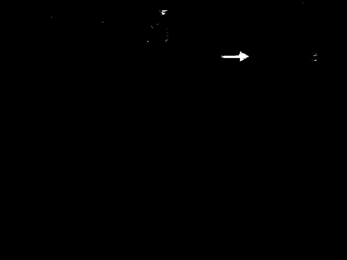
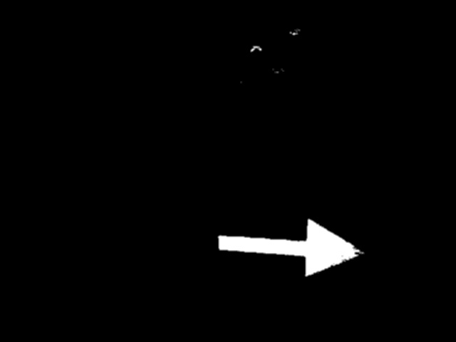
Step 3: Not only the red, but also the white pixels are filtered out. In other words the HSV image is tresholded which results in a binary image. This tresholding is done in a certain range of minimum and maximum values for the hue (H), the saturation (S) and the lightness value (V). Because red is both on the left and the right side of the color range, red tresholding is done for two different ranges to capture the whole red spectrum. Tresholding for the different ranges of red is combined to one binary image with the function bitwise.or. Only one range is necessary when tresholding for white pixels. The result of the white tresholding is saved separately. As example, the red tresholded picture looks as follows:

Step 4: The binary image gives the different red spots a little bit frayed contours. Therefore the image is blurred, in other words the contours are smoothened and some pixels are filled up to create a fully padded area. This is done with the floodfill algorithm, which works a bit like a minesweeper game. A kernel size of 3X3 is used, which gives sufficient smoothened contours. This results in the following picture:

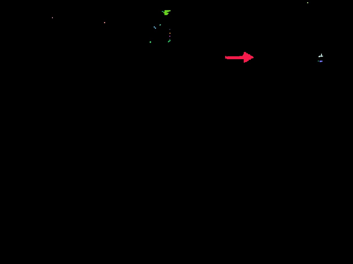
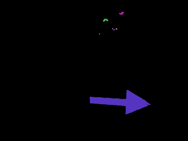
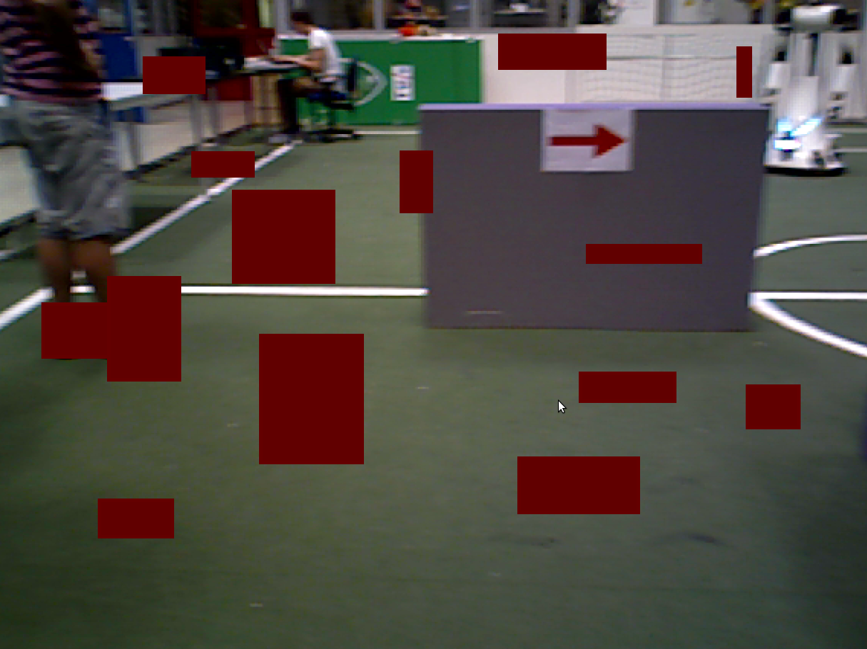
Step 5: With the OpenCV option findcontours the different contours of all the red blobs are found. All the contours are saved as a vector in the vector contours. For each founded contour, the corresponding blob is coloured differently. This results in the following picture:

If the size of the vector contours is larger than zero the following steps are performed:

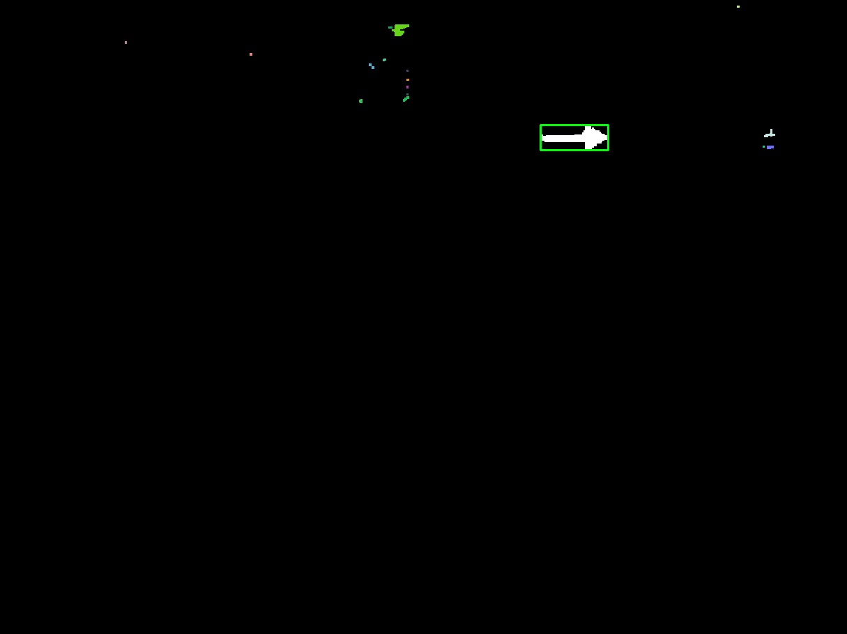
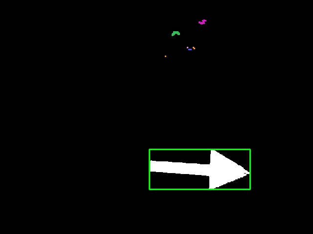
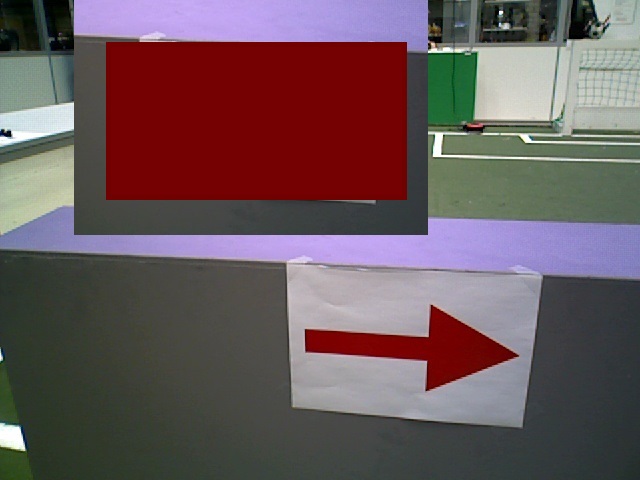
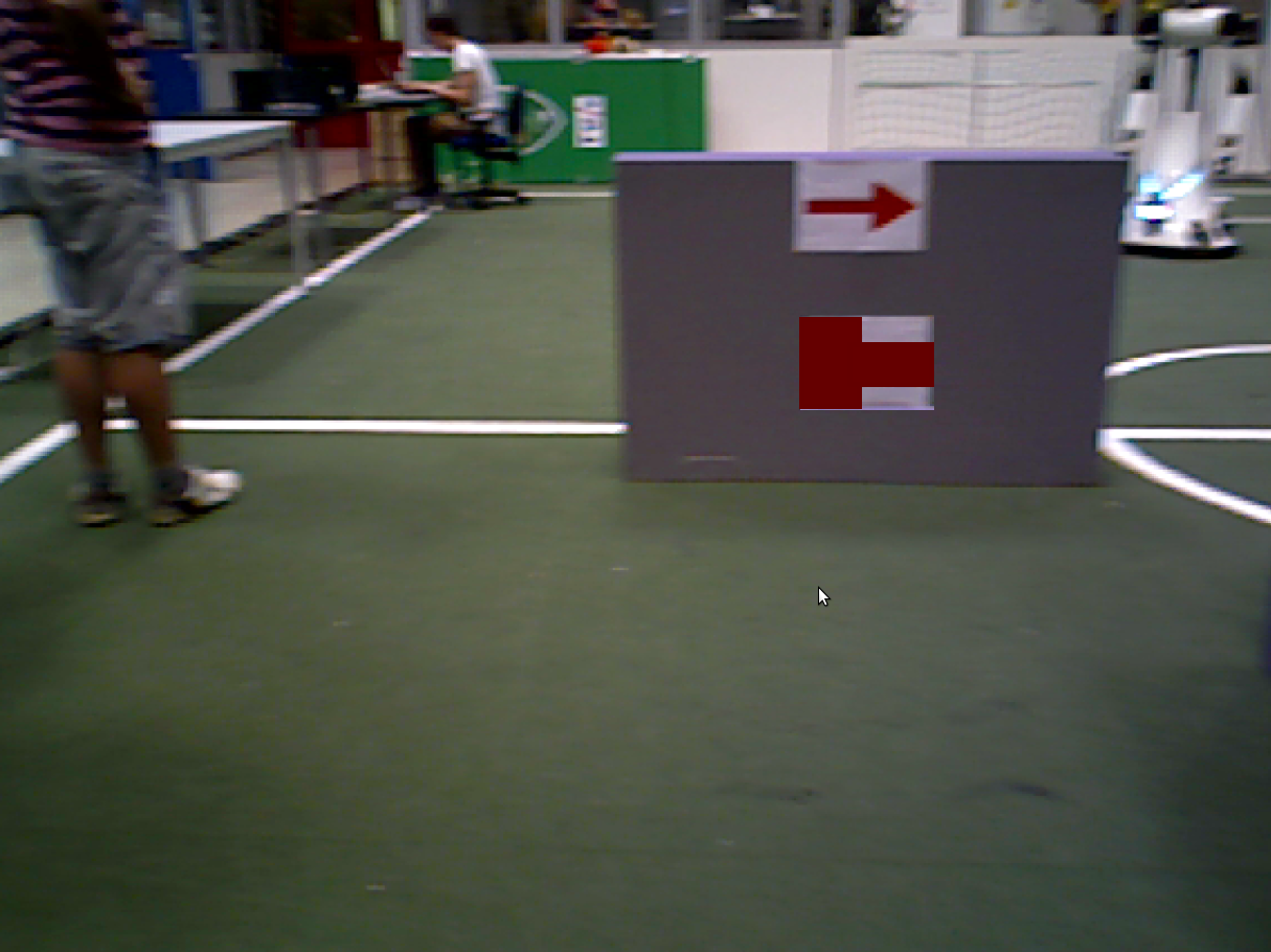
Step 6: Now the areas inside all different contours are calculated with the OpenCV function contourArea. With a loop the largest area is determined. The largest contour index is stored. When the largest area is found, a closest rectangle is drown around the area with the option boundingRect. This results in the following picture:

Step 7: The largest area counts the number of dots of the arrow. A minimum number of dots is set, to determine if an possible arrow can be recognized. If the largest area is bigger than the minimum number of dots, the script preceeds with the next steps. Otherwise the founded contour is too small for accurate arrow recognition. Moreover, Pico is in this case very far from the arrow (> 8 metres) and may first become closer to the arrow before further image processing.

If the largest area is larger than a stated minimum number of dots then is preceded with next steps. Else an integer PossibleArrow = 0 is sended over a rostopic to let Pico know there is no large enough red blob detected and to preceed with next image.

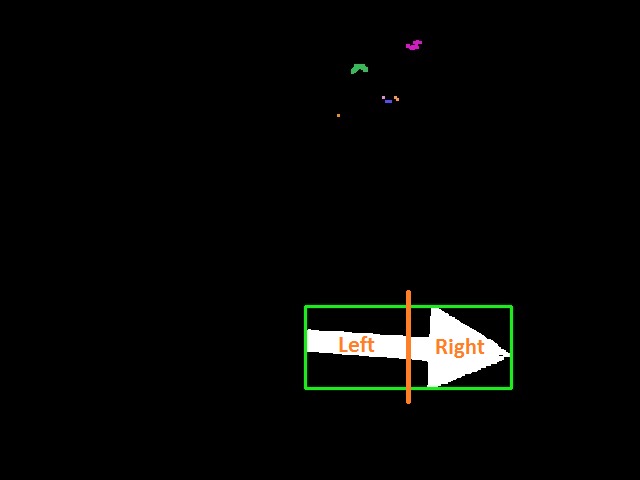
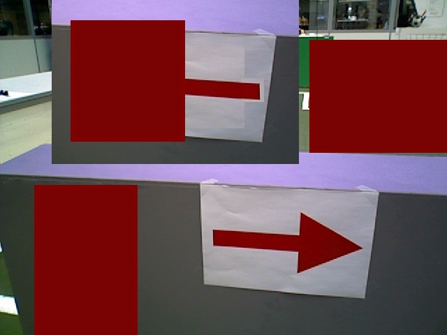
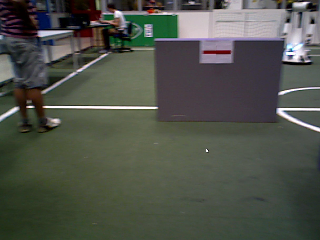
Step 8: The rectangle is now divided in two equal parts, a left and a right part. This is done by creating two different ROI’s (Regions of interest) on base of the coordinates of the rectangle. The x-range of the left part is bounding_rect.x until bounding_rect.x+0.5*bounding_rect.width. The x-range of the right part is bounding_rect.x+0.5*bounding_rect.width until bounding_rect.x+bounding_rect.width. The y-range of the left and right part are the same: bounding_rect.y until bounding_rect.y+bounding_rect.height. This can be visualised as follows:

Step 9: The number of red dots are calculated for the left part as well as the right part. Moreover, the number of white dots is calculated for the whole rectangle. With this information is determined if an arrow is recognized and to which side the arrow is pointed. The detection of the arrow is determined by the ratio of the red dots between left and right. The ratio must be larger than 1.5 to detect an arrow. Moreover there must be a minimum number of white dots in the rectangle too. This makes the script more robust for red objects in the surroundings as a white t-shirt or a chair for axample. Three different situations may occur:

• Situation 1: If number of red dots right > 1.5*Number of red dots left AND number of white dots > minimum number of white dots.

If this situation occur an arrow to the right is detected and integer PossibleArrow=1 is sended over the topic. In addition, there is checked whether Pico is allready close enough to the arrow to set his target point to the direction of the arrow. The largest area must be larger than a number of pixels. If this is the case, integer PossibleArrow is changed to 3.

• Situation 2: Else if number of red dots left > 1.5*Number of red dots right AND number of white dots > minimum number of white dots.

If this situation occur an arrow to the left is detected and integer PossibleArrow=1 is sended over the topic. In addition, there is checked whether Pico is allready close enough to the arrow to set his target point to the direction of the arrow. The largest area must be larger than a number of pixels. If this is the case, integer PossibleArrow is changed to 2.

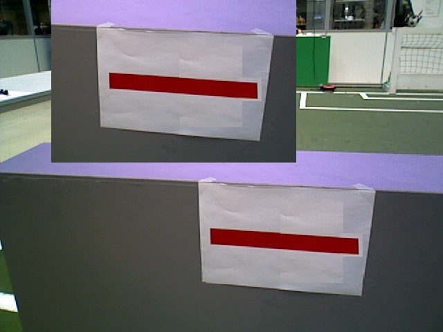
• Situation 3: Else ratio between red dots left and right is not large enough AND/OR number of white dots is smaller than minimum.

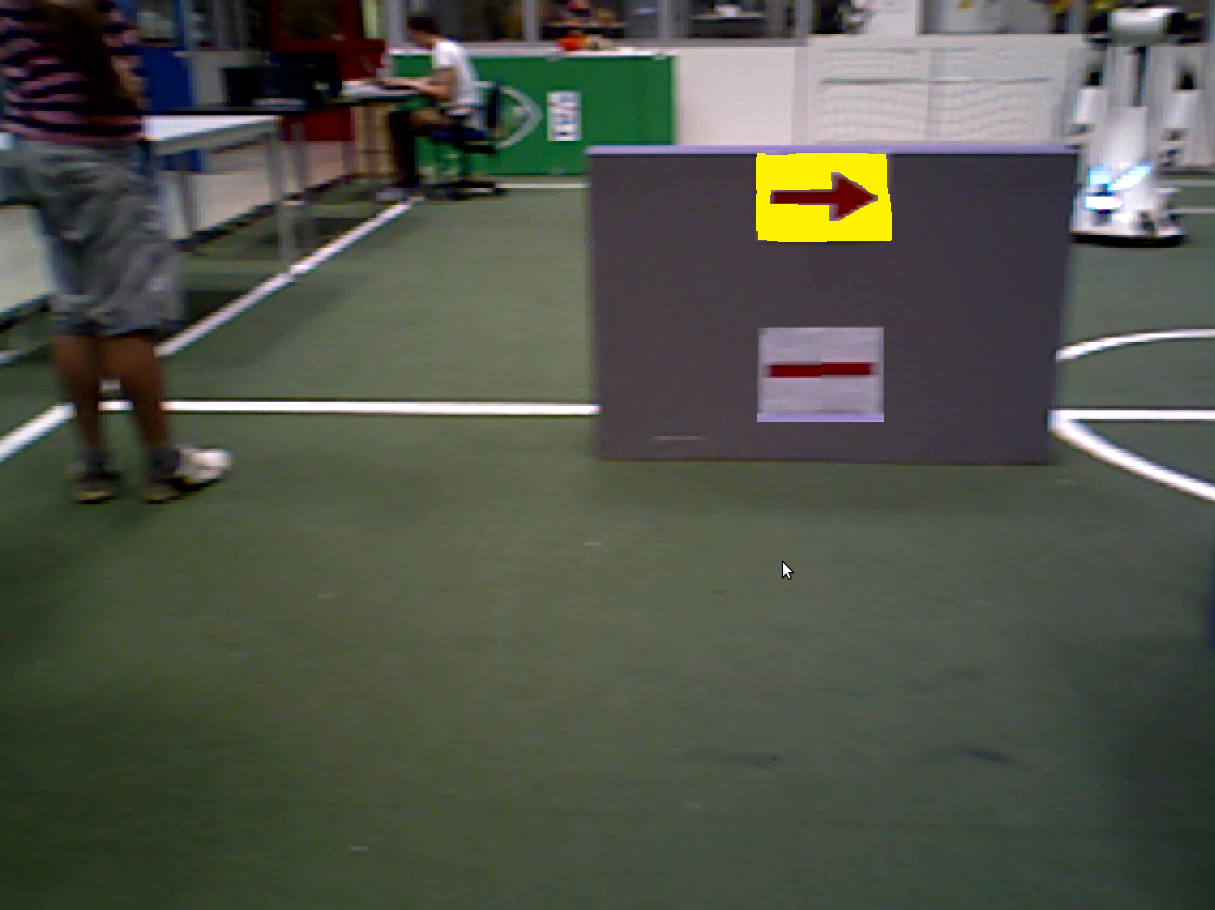
If this situation occurs, the possible arrow was unfortunately not an arrow and PossibleArrow is changed back to 0. The contour with the largest contour index is erased from the vector contours. However, not the whole contour is erased, but one point is left in the contour. This small contour consisting of 1 point ensures that there are know problems when calling the index of the contour. It gives no unwanted results, because this contour has an infinitesimal contour area. Steps 6 to 9 are performed again for the second largest surface. If still no arrow is found than again for the third largest surface, and so on until no contours are left or the largest area is smaller than the mimimum number of dots.

Step 10: Once the arrow is detected and its direction is verified, the main node must be told. This is done by sending an integer over a ROS-topic:

0: No arrow detected

1: Small (faraway) arrow detected

2: Large (near) left arrow detected

3: Large (near) right arrow detected

Testing script:

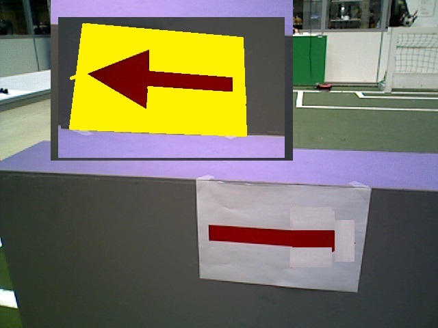
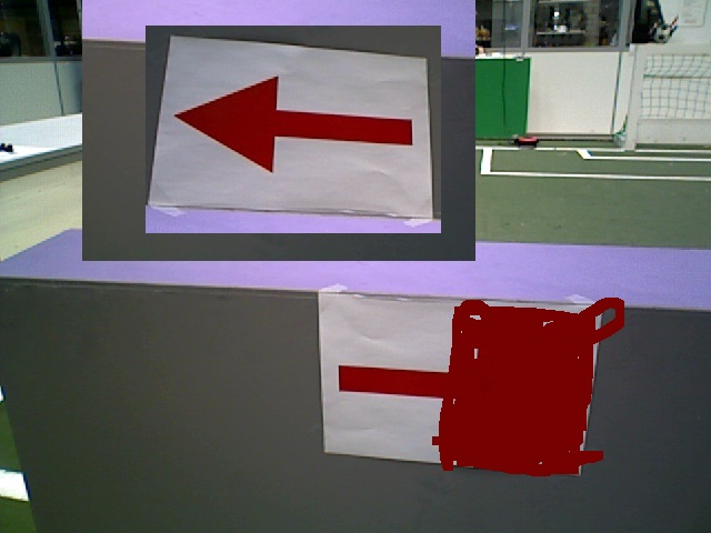
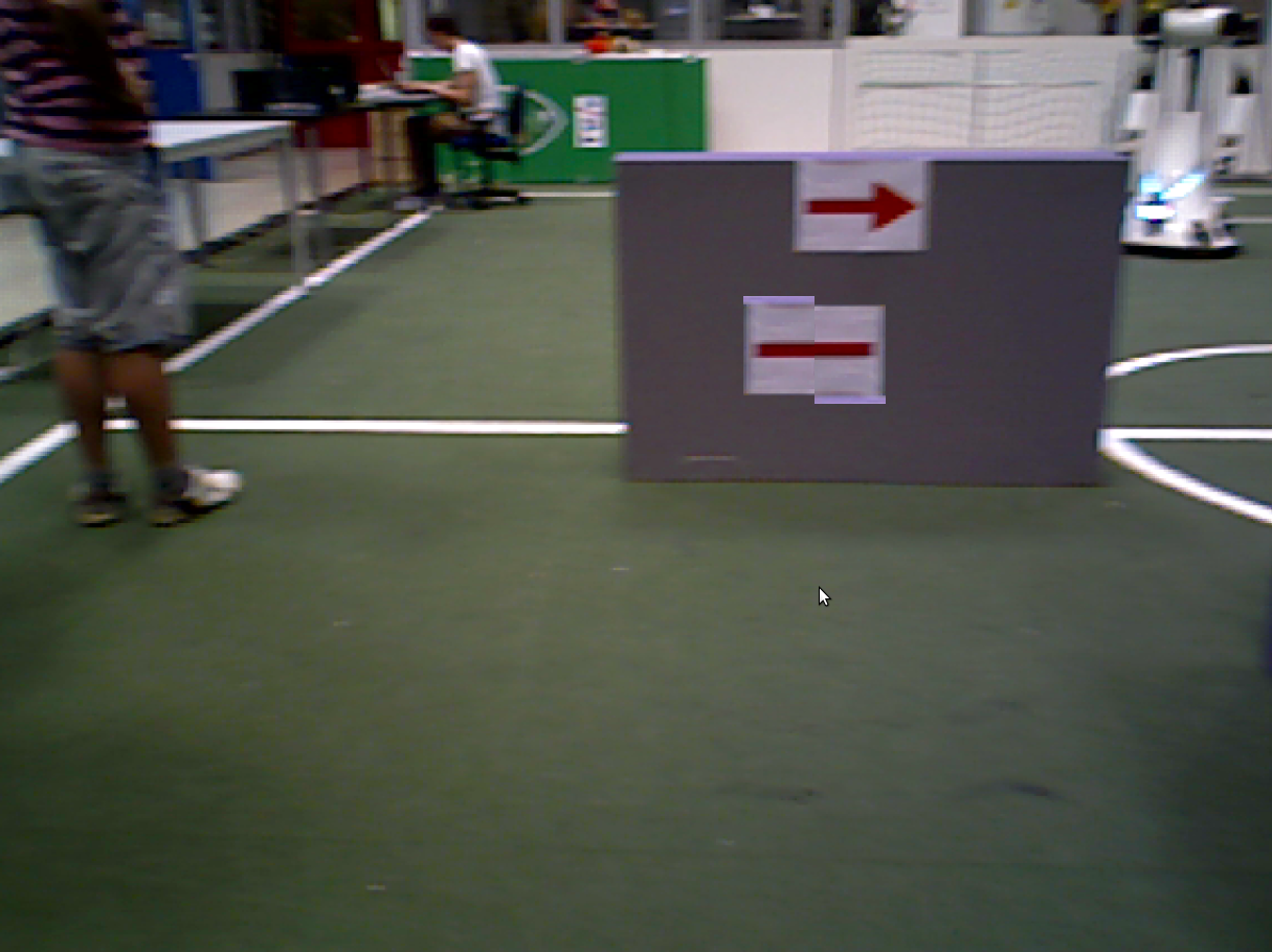
This scripts is tested by running for images in which different situations may occur.

This figures are edited printscreens from a recorded bagfile. Further finetuning of the parameters and testing of the communication over the topic is done while running the script for the whole bagfile.

World recognizer

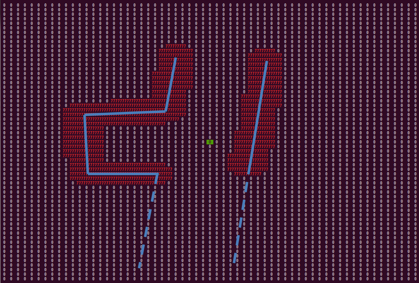
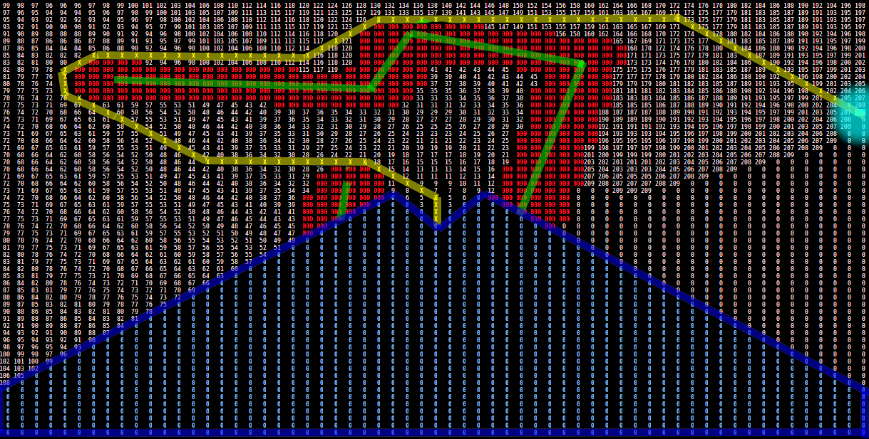
The 'World recognizer' function converts the laser data provided by the 'Laser node' to a matrix used in the 'Shortest path algorithm' function. This matrix contains all areas pico is not allowed to go. The matrix represents a square grid around pico. The amount of cells and cell size are determined before hand. A zero in the matrix means that the respective cell is unoccupied. Each point of the laser data array is transformed to a position in the grid, and every cell in a safety circle with a diameter of 5 cells around this point are marked as occupied. Walls get the number 777 assigned to their cells. Assigning walls with a distinct number allows for easier human reading and coloring options. The safety circle is added to maintain a distance between the walls and the optimal path, and to ignore small gaps as possible corridors. In the picture below, an example of the matrix with detected walls is shown.

The walls are represented by the blue line's which are dotted for walls outside pico's vision range. The occupied matrix cells are depicted by the number 777, colored red. The 0 with the green rectangle is the position of pico. As can be seen, angle's of 90 degree are not depicted as such, which can be caused by inaccurate laser data, scaling errors, or inaccuracies in the laser range detectors specifications. However, slight curving of walls does not in navigational errors, and is thus of little importance.

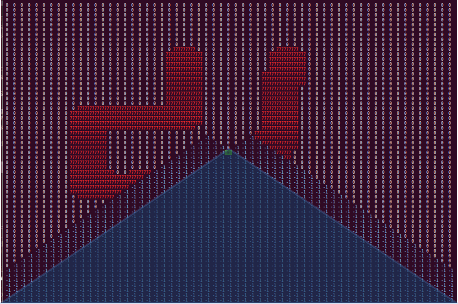
To prevent pico from driving to his blind spot, all non visible cells are marked as occupied, this time with the number -1. Again, a distinct number for each kind of occupation allows for easier reading and coloring of the matrix. The physical blind spot is expanded by a region on each side, to prevent pico from turning back into the corridor he came from. These artificial blind spots have the added benefit of initiating a deadlock when pico is driving head first into a wall. How this deadlock works is explained in the section about the optimal path algorithm. In the image below, the matrix is shown with blind spots.

Again, the red numbers 777 indicate that a grid is occupied by a wall, and the 0 with green rectangle is pico's position. In addition, each blue -1 represents a cell in the blind spot. The highlighted area in the blind spot is pico's natural blind spot and the non highlighted areas are the artificial blind spots.

Shortest path algorithm

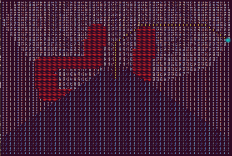
The matrix provided by the 'World recognizer' function is used in the 'Shortest path algorithm' function to determine the optimal path with the use of a modified version of Dijkstra's algorithm. The algorithm starts at pico's position, and looks if the adjacent cells, including diagonal ones, are occupied. In the grid matrix, every adjacent cell with a zero will be occupied, changing the zero for a cost number. The cost number is dependent on how long the path it belongs to is. The shortest path available, thus with the lowest cost number, is the first to be expanded. A horizontal or vertical move adds a cost of two, and a diagonal move a cost of 3. The expansion of paths is looped until the target point is encountered. The target point is represented by a 999 in the matrix, and is placed either above pico, to the right and slightly above, or to the left and slightly above, depending on which target direction has been received from the 'Image recognition node'. In the image below, a the matrix containing the walls and blind spots is depicted after the path finding algorithm.

In this image, the red 777's are again the walls, the blue -1's are the blind spots, the 999 is the target point, in this case for the right hand rule, and the white numbers are the pathing costs. The yellow crosses represent the optimal path.

The pathing algorithm has some additional features. The most important one is the already mentioned deadlock. When no optimal path can be found for two consecutive iterations, pico initializes a 90 degree turn in the opposite direction of the target point. This does also occur when pico gets stuck. Furthermore, the walls are inflated, as mentioned before, which means that small gaps are not seen as corridors. The path finding algorithm runs twice per second, and outputs a desired direction vector, which is the vector describing the distance between the 5th pathing point and the first pathing point, which is located at pico's position. This point should represent the direction pico should drive to follow the beginning of the path. The fifth point is chosen because it is a compromise between the advantages of the first few points and points further down the path. Points close by have a very large angle increments, for example 45 degrees for the second layer. Points further down the path run the risk of ending up at the other side of walls, in case the path wraps around a wall. Since walls are at least 5 cells wide, this is not possible with the 5th point.

Collision avoidance

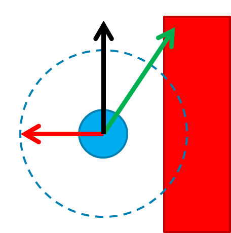
The "Collision avoidance' function checks the desired direction, provided by the 'Shortest path algorithm' function, for collisions and, if necessary, alters the desired direction. To check for collisions, pico checks the laser data array for the closest laser data point. If this point is within 0.38m of pico, a correction vector is created, pointing away from said closest point. The closer this point is to pico, the larger the correction vector. The desired direction vector and correction vector are then added together to obtain the final direction vector, which is then scaled to 0.2m/s. This mechanism acts like a one way p controller. In the picture below, the principle of the collision avoidance is illustrated.

In this picture, pico is represented by the blue dot,the range of 0.38m is represented by the blue dotted circle, and the red rectangle represents the wall. The green arrow depicts the desired direction vector, the red arrow is the correction vector and the black arrow is the final direction. Please note that this image has objects with arbitrary size, and are thus not scaled properly.

Additional functions

A couple of additional functions, not worth their own block in the diagram, have been implemented.

Entrance detection

When the code starts to run, pico's target point is set in the upper middle of the matrix. Once pico encounters walls behind his y axis, or a certain time has passed, the target point is set to the default position. This is done to prevent pico from driving in circles outside the maze.

Exit detection

Once pico encounters no walls within two meters in a angle of 90 degrees to the front, his target point is set to the upper middle of the matrix, prompting pico to drive straight forward. Once there are no walls within 2 meters in pico's vision range, the maze is completed, and pico commences a victory dance.

Corridor competition

The code used for the corridor competition featured two main features: collision avoidance and intersection detection (see above). The collision avoidance algorithm is always running to correct the drive direction in case Pico is too close to a wall. The intersection detection only runs until an intersection is found, as the corridor will only have 1 exit. If a corridor to the left or right is detected, Pico will turn in that direction and continue driving forward until he has completely exited the corridor. The collision avoidance remains live in order to prevent Pico from hitting any walls during the departure from the corridor.

Evaluation

Pico was able to navigate out of the corridor. However, it was not flawless. The corridor exit was detected before Pico was in the middle of the exit. After turning Pico was not unable to drive through the exit without hitting a wall and the collision avoidance had to correct Pico's movement. This could have been prevented by placing the detection range more towards the rear of Pico. Additionally another check could be implemented to keep Pico driving forward until the middle of a corridor is detected before stopping and turning.

Eventually the 'look around-decide-turn' approach was abandoned in favor of an integrated path planning algorithm. By using path planning, Pico can look around and drive towards a certain point simultaneously while keeping a safe distance from the walls at the same time. For robustness reasons, the collision avoidance will remain in place.

Final maze competition

First attempt

We had multiple versions of our script ready for the competition. The versions varied from the most basic navigation script, without entrance and exit detection, victory dance and arrow recognition, to the version with all features enabled. The maze of the competition turned out to be relatively simple, but well designed to test each feature required for optimal driving. Therefore, we knew we would not win without the arrow detection, which was not tested in real life yet, and had questionable robustness during simulations. Because we had, and still have, full confidence in the navigational algorithm itself, we opted to run our first try with arrow detection enabled. While it seemed to work momentarily, the script lost track of the first arrow, prompting pico to take the wrong turn. At the end of the corridor, pico correctly detected the deadlock, and started turning. However, during the turn, an unidentified object, most likely the red door, was detected as an arrow. This put the target point at the left side, changing the deadlock turn direction to negative. After turning back a little, the door was out of sight, resetting the turn direction to positive. This process seemed to repeat itself a couple of times, so we elected to abort this attempt.

Second attempt

During the second attempt, we opted to run the script in its most basic version, since entrance detection was not needed. Furthermore, our victory dance could not be performed either, since there was no room available and pico would be turned of once he would cross the finish line. Since we had no arrow detection this time, pico turned to the wrong direction at the first arrow. Once the dead end was in his vision range, pico turned successfully and finished the maze without any further mistakes. The trust in our core navigation turned out to be justified. The end time was 1 minute and 23 seconds, resulting in a respectable fifth position.

Evaluation

The maze challenge went more or less as expected. We had serious doubts about the robustness of the arrow detection, and with only half of the red color range properly implemented, it would be questionable whether or not pico could even read the arrow. It turned out to be the worst of both cases. Pico could not read the arrow, but another object, most likely the door, was detected as an arrow a few moments later. The lackluster performance of the arrow detection was partially compensated by the effectiveness of our navigator. The high level navigation, calculated with Dijkstra's algorithm, immediately detected any dead ends, and always sent pico to the corridor deemed optimal by the selected maze solving strategy. The simple, yet effective low level navigation kept pico around the middle of the corridor, and led the robot around corners in a smooth, curved manner. With the exclusion of the dead end turn, pico never stood still, always moving at maximum velocity. The excellent performance of our navigator enabled us to take the 5th spot, above multiple groups with successfull arrow detection.

Path Planning

The intersection based navigation system only works for perfect situations. In order to make the navigation more robust and able to tackle more complicated situations, a shortest path finding algorithm is implemented.

Wall detection and representation

The navigation algorithm uses a matrix to represent the local area around Pico. Collect laser data is placed inside this matrix. The detected walls are inflated to make sure that Pico does not recognize small openings between wall sections. The inflation layer is also used to give the planned path a certain distance parallel to the wall.

Target point location

Pico will be provided with three possible target points: Straight ahead, upper left or upper right. If no arrow is detected, the primary direction places the target point left or right. The arrow recognition will communicate if an arrow is detected. If an arrow is seen in the distance, the target is set to straight ahead. If Pico is close enough to an arrow, the arrow determines the target point location.

Shortest path algorithm

The empty cells in the matrix are now filled with numbers that correspond to the cost (in terms of distance) of driving to that cell. Using Dijkstra's algorithm, the cheapest path is selected. The found path is used to determine the direction vector.

The process is repeated with a frequency of 2 Hz.

Addition of blind spot

As Pico is going around a corner, the old corridor might be seen as the shortest path. To prevent this, an artificial blind spot is added behind and slighty left- and right-behind Pico to prevent Pico from turning back into the previous corridor.

Path planning matrix example

Below is an image representing the matrix during the path planning stage.

-Green: detected walls

-Red: inflated walls

-Blue: blind spot

-Light Blue: target

-Yellow: shortest path

-White numbers: path cost