Embedded Motion Control 2014 Group 1

Group Info

Name:	Student id:	Email:
Groupmembers (email all)
Sander Hoen	0609581	s.j.l.hoen@student.tue.nl
Marc Meijs	0761519	m.j.meijs@student.tue.nl
Wouter van Buul	0675642	w.b.v.buul@student.tue.nl
Richard Treuren	0714998	h.a.treuren@student.tue.nl
Joep van Putten	0588616	b.j.c.v.putten@student.tue.nl
Tutor
Sjoerd van den Dries	n/a	s.v.d.dries@tue.nl

Meetings

Weekly meetings are planned during the course. Every Wednesday a standard meeting is planned to discuss progress with the group and with the tutor. Presentations from these weekly meetings can be found with the presentation links below. Important meeting decisions can be found with use of the meeting liks below. Next to the standard weekly meetings evening meetings are planned to work as a group on the software design. For some meetings the minutes can be shown by clicking on the hyperlinks below.

1. Meeting - 2014-05-02
2. Meeting - 2014-05-12
3. Meeting - 2014-05-14
4. Meeting - 2014-05-15
5. Meeting - 2014-05-16
6. Meeting - 2014-05-21
7. Meeting - 2014-05-23
8. Meeting - 2014-05-27
9. Meeting - 2014-05-28
10. Meeting - 2014-06-02
11. Meeting - 2014-06-04
12. Meeting - 2014-06-05
13. Meeting - 2014-06-06
14. Meeting - 2014-06-11
15. Meeting - 2014-06-13
16. Meeting - 2014-06-18
17. Meeting - 2014-06-20
18. Meeting - 2014-06-25
19. Meeting - 2014-06-27
20. File:Presentatie week 3.pdf
21. File:Presentation week 4.pdf
22. File:EmbeddedMotionControl01 wiki.pdf

Time Table

Fill in the time you spend on this course on Dropbox "Time survey 4k450.xlsx"

Planning

Week 1 (2014-04-25 - 2014-05-02)

• Installing Ubuntu 12.04
• Installing ROS
• Following tutorials on C++ and ROS.
• Setup SVN
• Plan a strategy for the corridor challenge

Week 2 (2014-05-03 - 2014-05-09)

• Finishing tutorials
• Interpret laser sensor
• Positioning of PICO

Week 3 (2014-05-10 - 2014-05-16)

• Starting on software components
• Writing dedicated corridor challenge software
• Divided different blocks
  • Line detection - Sander
  • Position (relative distance) - Richard
  • Drive - Marc
  • Situation - Wouter
  • State generator - Joep
• File:Presentatie week 3.pdf

Week 4 (2014-05-17 - 2014-05-25)

• Finalize software structure maze competition
• Start writing software for maze competition
• File:Presentatie week 4.pdf

Week 5 (2014-05-26 - 2014-06-01)

• Start with arrow detection
• Additional tasks
  • Arrow detection - Wouter
  • Update wiki - Sander
  • Increase robustness line detection - Joep
  • Position (relative distance) - Richard
  • Link the different nodes - Marc

Week 6 (2014-06-02 - 2014-06-08)

• Make arrow detection more robust
• Implement line detection
• Determine bottlenecks for maze competition
• Make system more robust

Week 7 (2014-06-09 - 2014-06-15)

• Implement Arrow detection
• Start with more elaborate situation recognition for dead end recognition
• Test system

Week 8 (2014-06-16 - 2014-06-22)

• Improve robustness
• Finish dead end recognition

Week 9 (2014-06-16 - 2014-06-22)

• Improve robustness of system for maze competiotion

Corridor challenge

For the corridor challenge a straight forward approach is used which requires minimal software effort to exit the corridor succesfully.

Approach

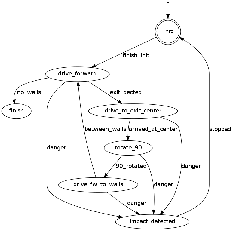
For PICO the following approach is used to solve the corridor challenge.

• Initialize PICO
• Drive forward with use of feedback control
  • Position [math]\displaystyle{ x }[/math] and angle [math]\displaystyle{ \theta }[/math] are controlled
  • A fixed speed is used, i.e., [math]\displaystyle{ v }[/math]
  • Safety is included by defining a distance from PICO to the wall, where it will stop if the distance becomes [math]\displaystyle{ \lt 0.1 }[/math]m
  • The distance between the left and right wall is calculated. With use of feedback pico will always be controlled to stay in the middle of the corridor.
  • The angle of pico relative to the walls is used to keep PICO oriented in the same as the walls.

• If no wall is detected feedforward control is used
  • Drive for [math]\displaystyle{ T_e }[/math] [s] after no wall is detected
• After [math]\displaystyle{ T_e }[/math] [s] PICO rotates +/-90 degrees using the odometry
  • +/- depends on which side the exit is detected
• Drive forward with use of feedback control
• Stop after [math]\displaystyle{ T_f }[/math] [s] when no walls are detected

States PICO corridor challenge

The states of PICO for the corridor challenge are visualized in the following figure:

Result

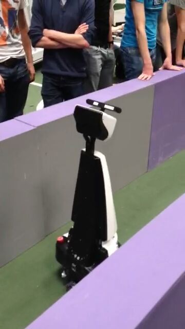
First place!!

Maze challenge

Maze solving algorithm: the wall follower

The choice for this algorithm is based on the fact that its simple, easy to program but nevertheless effective.

Working principle:

The starting point of this algorithm is that the mobile robot starts following passages and whenever a junction is reached it always turn right (or left). Equivalent to a human solving a Maze by putting their hand on the right (or left) wall and leaving it there as they walk through. This algorithm will be improved by adding arrow detection and dead end recognition.

Examples

Examples of a maze solved by the Wall follower algorithm are shown below.

• Link 1
  
• Link 2
  

Software architecture

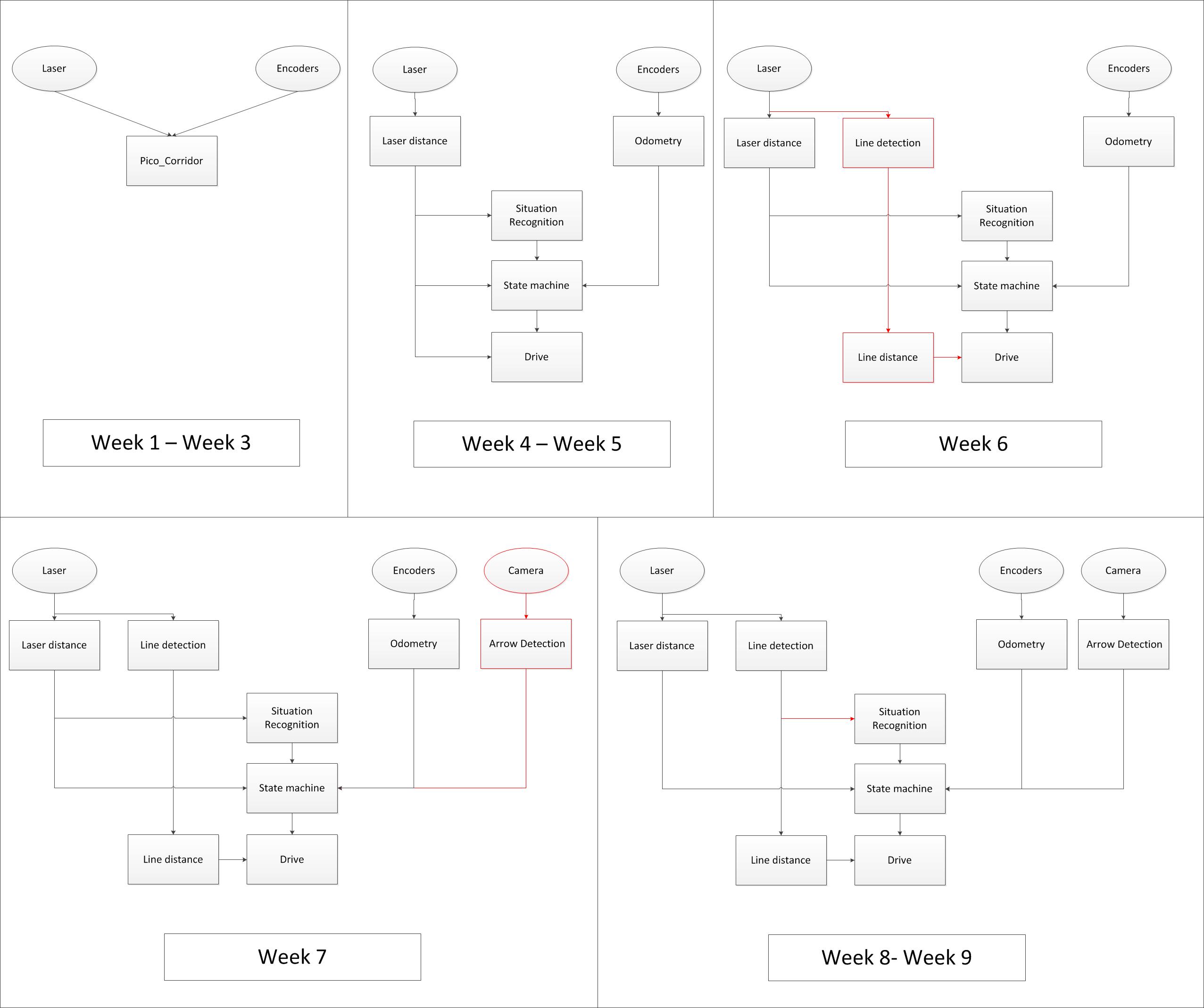
The figure below shows how the software architecture changed during the course (click on picture to enlarge). Eclipse blocks represent sensor data and rectangular blocks represent ROS nodes. The first three weeks one node is used for the corridor challenge. After this the new architecture was implemented and improved over the weeks. Most important are the addition of the line and arrow detection. Furthermore it becomes clear that the line detection replaced most of the laser distance.

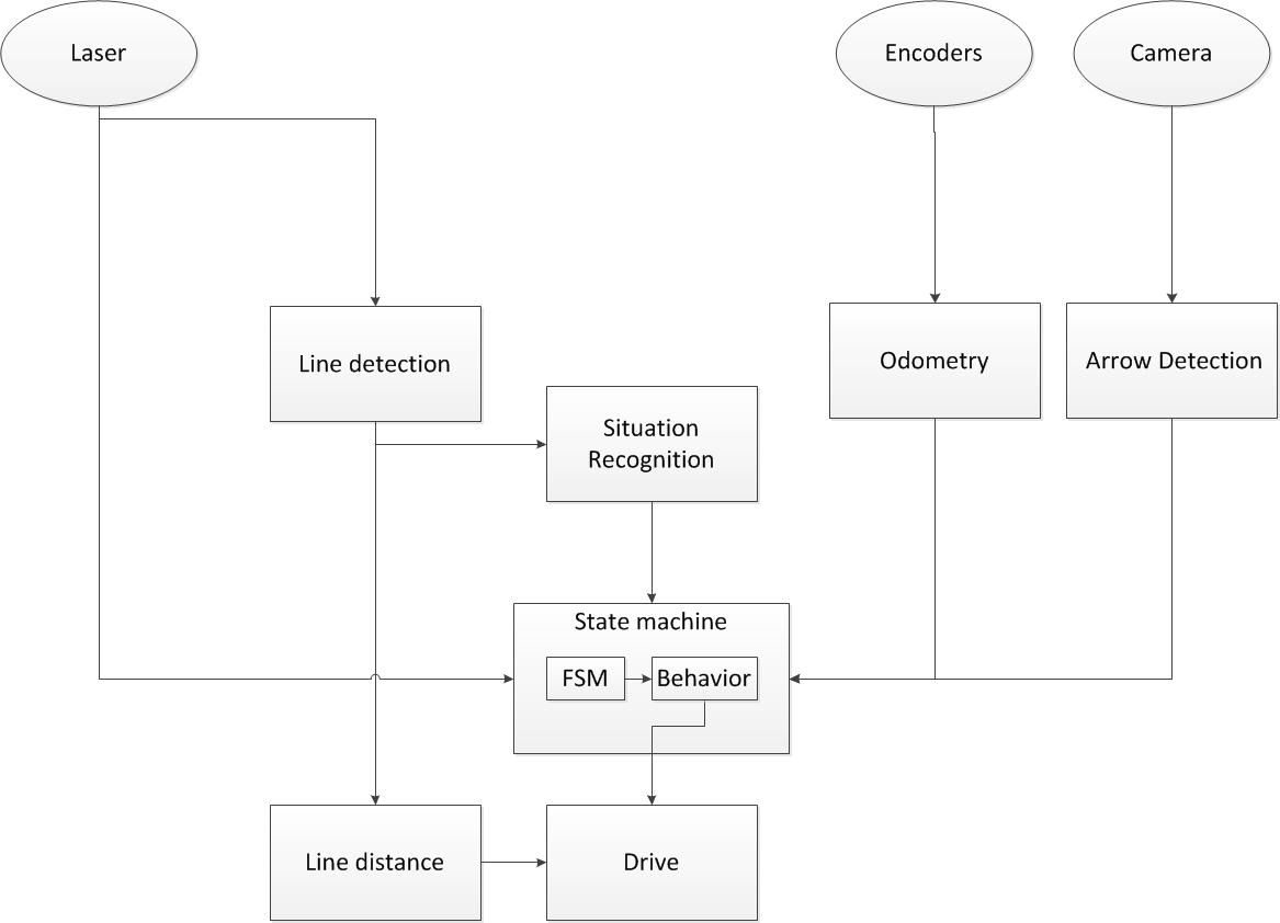
An enlarged picture of the final software architecture is shown below.

Based on the incoming laser data from Pico lines are generated with use of a hough transform. With use of the line data situations are recognized. In this architecture situations are for example exit left, exit right and dead end. This information is send to the state machine. Next to the situation recognition also information about a detected arrow is send to the state machine, this gives simply information if there is an arrow to the left or right. Whit this information it is determined what kind of behavior is needed in the given situation. An example could be that the robot needs to turn 90 degrees to the right because a t-junction is recognized. The state machine sends the command to rotate the robot with a given speed untill the odometry shows that the robot has turned 90 degrees.

The needed behavior of the robot is send to the drive process which sends the velocities to PICO. The drive block also makes sure that the robot drives in the middle of the maze corridors and has an orientation perpendicular to the driving direction. This is also done with the line input. Dependent on the state of the robot this control is on or off.

The laser distance block which is an input for the state machine is only used for 'safe drive'of PICO. When an object is detected on a certain threshold PICO will go to its safety state.

I/O structure

The different components that are visualized in the software architecture scheme are elaborated here

Node	Subscibes topic:	Input	Publishes on topic:	Output	Description
Line detection	/pico/laser	Laser scan data	/pico/lines	Array of detected lines. Each line consists out of a start and an end point (x1,y1),(x2,y2)	Transformation of raw data to lines with use of the Hough-transform. Each element of lines is a line which exists out of two points with a x- y and z-coordinate in the Cartesian coordinate system with Pico being the center e.g. (0,0). The x- and y-axis are meters and the x-axis is the front/back of Pico while the y-axis is left/right.
Arrow detection	/pico/camera	Camera images	/pico/vision	Arrow detected to the left of the right	Detection of arrows pointing to left or right.
Odometry	/pico/odom	Quaternion matrix	/pico/yaw	float with yaw angle	Transform Quaternion in roll, pitch and yaw angles. Only yaw angle is send because roll and pitch are zero.
Distance	/pico/line_detection	Line coordinates	/pico/dist	(y_left, y_right, x, theta_left, theta_right) also known as the 'relative position'	Determine distance to wall to left, right and front wall. Also determines angle left and right with respect to the walls.
Situation	/pico/line_detection /pico/laser /pico/vision	Line data, vision interpretation and possibly laser data.	/pico/situation	The situation where pico is in. For example corridor to the right, T-junction, etc.	Situation parameters.
State generator	/pico/situation /pico/yaw	Situation and yaw angle of Pico.	/pico/state	dx,dy, dtheta	Based on the situation Pico needs to go through different states and continue to drive. Every state defines an action that Pico needs to do.
Drive	/pico/state /pico/dist	(y_left, y_right, dy, x, dx, theta_left, theta_right,dtheta)	/pico/cmd_vel	Pico moving	Move pico in the desired direction

PICO messages

The different nodes are communicating with each other by sending Messages. Each nodes sends a set of messages with use of a publisher. The Message that are sends between the nodes are defined in this section.

Lines

The line message includes two points, p1=(x1,y1) and p2=(x2,y2), which are defined by the geometry messages package. A point consists of (x,y,z) coordinate. For points p1 and p2 the z-coordinate is set to zero.

Points p1 and p2 are connected to represent a line each line is stored in array:

  line[] lines

Duplicate lines are merged to one line. The detected lines are visualized as a Marker in rviz, by using the visualization_msgs package.

Vision

The vision message contains two booleans for if it either detects an arrow pointing to the left, or a arrow pointing to the right.

   bool arrow_left
   bool arrow_right

Distance

The distance message contains the following floats

   float32 YR
   float32 YL
   float32 THR
   float32 THL
   float32 X 

Determining the distances from pico to the detected walls.

Situation

Basically, there are eight main situations, these are shown in the figure below. If PICO does not detect any corner points, then it is located in a corridor. In this case the robot can go straight on. If PICO detects any corner points, then it might need to turn. Whether it needs to turn, depends on the situation. The different type of situations are

   Situation T-junction exit left right
   Situation T-junction exit front right
   Situation T-junction exit front left
   Situation Corridor
   Situation Corridor right
   Situation Corridor left
   Situation Intersection
   Situation Dead end

State generator

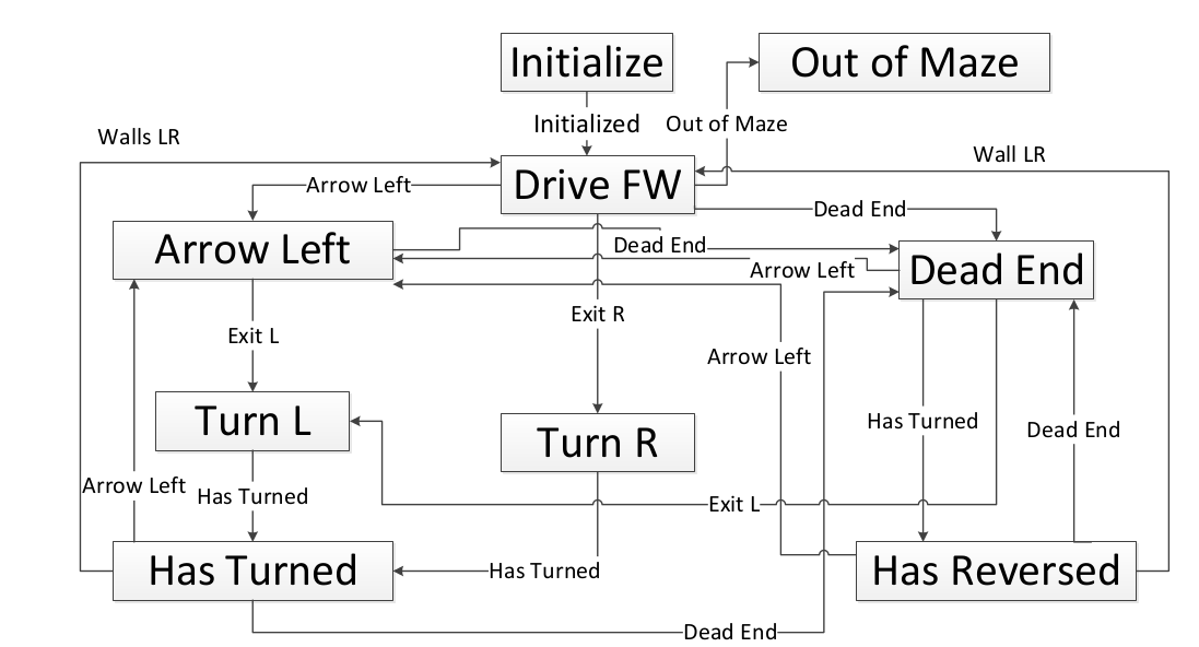
A Finite State Machine (FSM) is used to structure the decision making of pico. In an FSM, a set of states is defined in which specific behavior is described. The different state are denoted below

   State Initialize
   State Drive Forward
   State Arrow Left
   State Dead End
   State Turn Left
   State Turn Right
   State Dead End
   State Has Turned
   State Has Reversed

An overview of the different states and how they are connected will be illustrated in section Software components - State generator

Drive

The drive message sends commands to the drive node which actually sends the velocity commands to pico. The message contains two float32, one to specify the velocity forwards and one to represent the velocity by which Pico turns around his axis.

   float32 speed_angle
   float32 speed_linear

Software components

Line detection

Input: "/pico/laser"
Output: "/pico/lines"

Principle

Transformation of raw laser data to lines representing the walls of a corridor. This transformation is done with use of the Hough-Transform

Approach

• Convert laser data to points (x,y,z)
  
  • Transform from sensor_msgs::Laserscan to pcl::PointCloud<T>
• Convert PointCloud to 2d Matrix
  • Overlay grid, color each point white in the 2d image (CV::Mat)
• Apply Hough transform
• Transform lines in image coordinates back to world coordinates
  • Result: std::vector<CV::Vec4f> >
• Filter detected lines
  • Increases robustness by neglectin small gaps within the corridor

Arrow detection

Inputs: "/pico/camera"
Outputs: Booleans 'left arrow' or 'right arrow' on topic "/pico/vision"

Principle

The goal for the arrow detection block is to detect arrows in the corridor by using the asus xtion camera mounted on pico. Three different approaches/methods are considered to achieve this goal:

• Template matching: Template matching is a technique which tries to find the reference image in the current 'video-image'. The technique slides the smaller reference image over the current image, and at every location, a metric is calculated so it represents how “good” or “bad” the match at that location is (or how similar the patch is to that particular area of the source image). This was implemented using the openCV function matchTemplate, which results in a matrix with 'correlation' values from which a conclusion can be drawn where the template is matched best in the current image. See the following video:

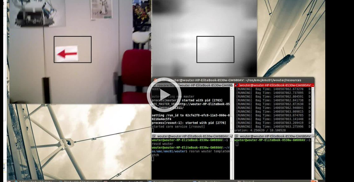
One problem of this technique is that only one 'reference' of a certain size is used to compare to the image, in our case with our dynamical changing 'size' of our to be detected arrow we are only detecting the arrow correctly if the size of the camera image of the error is exactly the size of the reference arrow. Therefore to make this method work in our case we need a lot of arrow-reference images of different sizes, which is not suitable.

• Feature detection: Another approach is to use algorithms which detect characteristic 'features' in both the reference and camera image and attempt to match these. Because these features are generally not scale or rotation dependent, this method does not run into the same problems as described for template matching. Therefore, this approach was investigated in the following way:
  • The OpenCV library contains several algorithms for feature detection and matching. In general, some steps are followed to match a reference to an image:
    • Detect features or 'keypoints'. For this several algorithms are available, notably the SIFT and SURF algorithms. Generally, these algorithms detect corners in images on various scales, which after some filtering results in detected points of interest or features.
    • From the detected features, descriptors are calculated, which are vectors describing the features.
    • The features of the reference image are matched to the features of the camera image by use if a nearest-neighbor search algorithm, i.e. the FLANN algorithm. This results in a vector of points in the reference image and a vector of the matched respective points in the camera image. If many such points exist, the reference image can be said to be detected.
    • Finally, using the coordinates of the points in both images, a transformation or homography from the plane of the reference image to that of the camera image can be inferred. This transformation allows tells us how the orientation has changed between the reference image and the image seen by the camera.
  • Implementation of the previously described steps resulted in detection of the arrow in a sample camera image. However, it was found that the orientation of the arrow could not accurately be determined by means of the algorithms in the OpenCV library. Due to the line symmetry of the reference arrow, a rotation-independent detector would match equally many points from the 'top' of the arrow to the top and the bottom of the arrow in the camera image, as the 'bottom' in the camera image could just as well be the top of the arrow had it been flipped horizontally.
  • One solution to the above problem could be to compare the vectors between the matched points in both images. Because it is only of interest whether the arrow is facing left or right, a simple algorithm could be defined which determines if many points which were located 'left' in the reference image are now located 'right', and vice versa. If this is the case, the orientation of the image has been reversed, allowing us to determine which way the arrow is pointing. However, this approach is probably quite laborious and a different method of detecting the arrow was found to also be suitable, which is why the solution described above was not pursued.

• Edge detection: By using the edge detection method, several steps are performed to recognize the edges of a red object within the camera image. Using those lines an eventual arrow can be detected. The steps are as follows:
  • Receive the rgb camera image.
  • Convert the rgb camera image to a hsv image.
  • This hsv image is converted to a binary image, red pixels are converted to white and all the other pixels are converted to black.
  • Using a floodfill algorithm the 'red' area is smoothened out, (8 connectivity is used)
  • Edge detection is applied, as an edge is a 'jump' in intensity it can be recognized, this is done using a canny edge detection algorithm.
  • By using a hough transform lines are fitted through the detected edges.
  • CombineLines function is used to 'neaten' the lines which are coming out of the hough transform, documentation is found at 'line detection' because exactly the same code is used.
  • By recognizing the slanted lines (of about 30 degrees) the arrow head can be recognized. And the direction of the arrow can be derived.

All the steps can been seen in the next video:

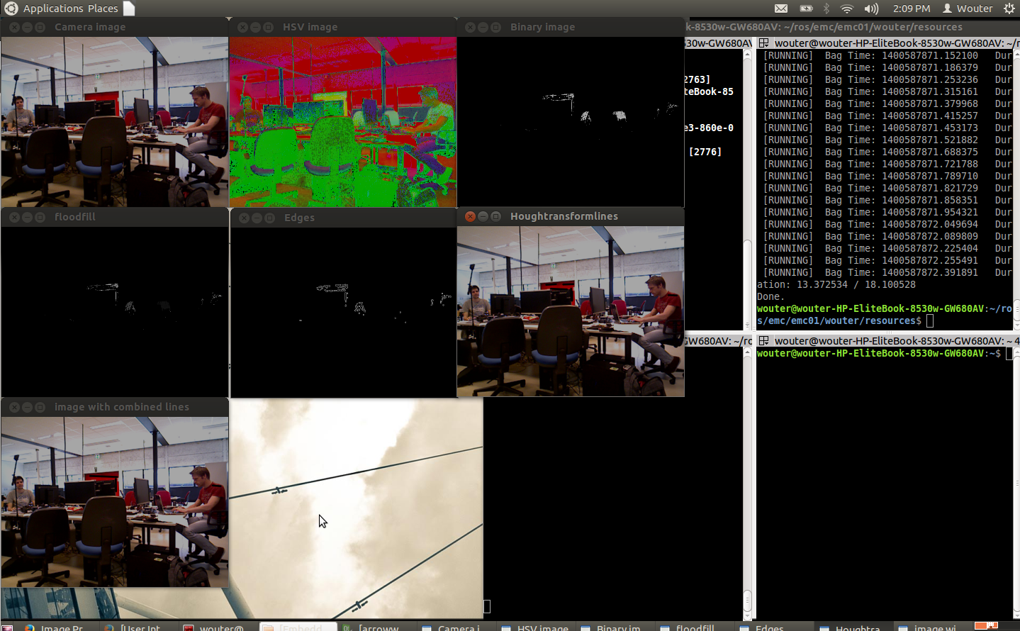
It can been seen that the arrow is recognized quite well and often, but to ensure some more robustness it is chosen to only create a boolean 'arrow detected' when at 3 adjacent frames the same arrow is recognized.

Relative distance

Inputs: "/pico/lines"
Outputs: "/pico/dist"

Principle

Determine distance to wall to left, right and front wall. Also determines angle theta with respect to the corridor

Approach

The input for this node are multiple points and every set of two points (x1,y1 and x2,y2) descibe a line. To get the calculation of the distance to that line right the first step is to check what the orientation of the line is. We want to determine wheter the first point or the second point from the line closest to pico. This is done very easy with the next piece of code:

       x1 = markers.points[i].x;
       y1 = markers.points[i].y;
       x2 = markers.points[i+1].x;
       y2 = markers.points[i+1].y;

       if (xx1>xx2){
           x1 = markers.points[i+1].x;
           y1 = markers.points[i+1].y;
           x2 = markers.points[i].x;
           y2 = markers.points[i].y;
       }

So in this situation the first point (x1,y1) is always in x-direction closest to pico.

For every line the angle theta can be calculated with the next fomula:

[math]\displaystyle{ \theta = atan((y2-y1)/(x2-x1)) }[/math]

The position perpendicular to the line/wall is calculated with the next formula:

[math]\displaystyle{ Y = y2 - ((y2-y1)/(x2/x1))*x2*cos(\theta_1) }[/math]

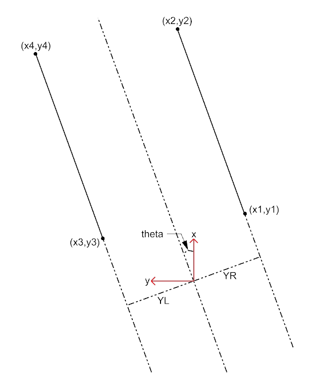
This formula extends the line till next to pico, so a line that is in front of pico also results in a value for Y (left or right) as if the line is next to pico. This is very usefull when pico has turned and is not between the walls yet. The definitions of the distances are visualized in the figure below. Note that in the figure only the angle with respect to the centerline of the coridor is given but the distance node will give the angle to the left and right wall separated.

The two formulas described above are calculated for every line. Based on the values resulting from those formulas the lines are filtered. the next filtering criteria are used:

• The absolute value of the angle theta must be smaller than 0.785 rad (45 degrees): this returns only the lines that are "vertical" (+ of - 45 degrees) for pico.

• When Y > 0 a line is left from pico.
• When Y < 0 a line is right from pico.

After these filtering steps is it still posible that multiple lines are detected to the left or the right of pico. So the next criteria was added:

• The line with the smallest Y value is used for the distance to the walls.

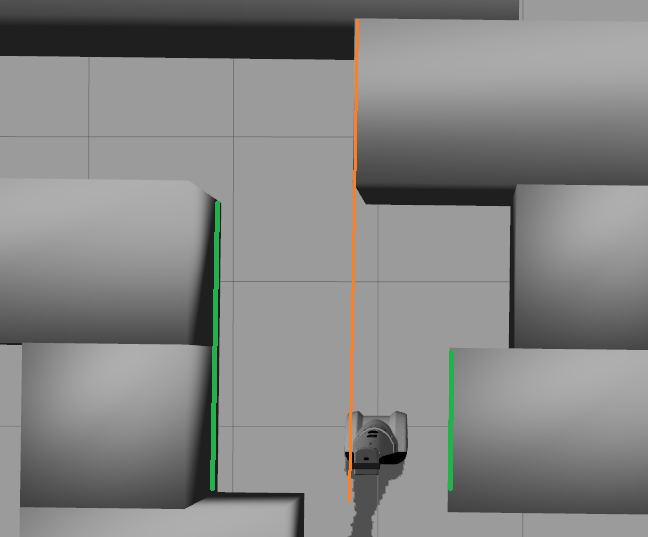
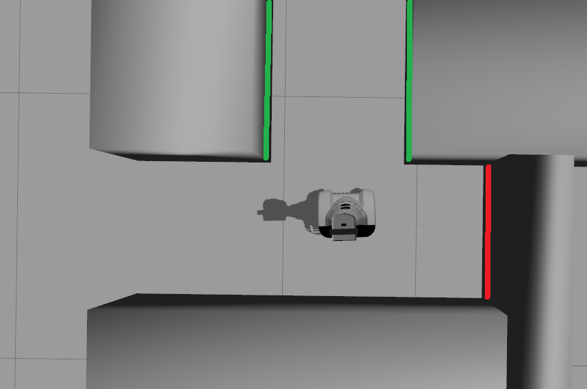
One critical situation when this approach might fail is shown in the Figure below. In that situation the wall in front of pico (orange line) has the smallest Y value, so the distance to the orange line would give Y_left. But because pico has only a few laser points on that wall it is not detected as a line so it wont give a problem and the distance relative to the two green lines will be returned.

Some other aproaches were also implemented and tested to do the filtering but the aproach mentioned above turned out to be the best option.

One other approach was to do the last filerting step based on the line with the x coordinate closesed to pico, so most of the time that is the line direct next to pico. This resulted in problems when pico turned towards a opening and a dead-end was left or right from pico as shown in the figure below. Pico would then calculate the distance to the left wall of the opening and the right wall of the dead-end (red line).

The outputs are defined as (Y_left, Y_right, X (forward), theta_left, theta_right).

Situation

Inputs: "pico/laser" "pico/lines" "pico/dist"
Outputs: Event that constains pico current situation of pico "pico/situation"

Principle

Determine the situation where pico is in. For example corridor to the right, T-junction, etc.

Approach

Two different approaches are taken into account, a simple approach in which only is detected if the left, front and right side of pico are 'free' of walls/obstacles. But also a more elaborate approach in which situations are detected like, junctions, T-junctions, crossings and dead ends. For the corridor challenge the simple approach is used, while for the maze challenge the more elaborated approach is be used.

Lines can be categorized in two types of lines:

• Longitudinal lines: y-coordinates of begin and end point are similar
  
• Lateral lines: x-coordinates of begin and end point are similar
  

Situations to be recognized:

• Inbetween two walls
  
  • No obstacles in front, no lateral line detected within X meter.
    
  • 2 longitudinal lines are detected.
    

• Junction
  
  • 3 lines are detected. From which two are longitudinal lines and one is lateral within (X meter).
    
  • Detect direction of juction by comparing the x -values of the longitudinal lines with the x-value of the lateral line.
    
    • Left junction: When the x value of the left line (the line with the smallest Y values) is 'minimum corridor width' smaller then the x value of the lateral line a gap on the left side is recognized.
      
    • Right junction: When the x value of the right line (the line with the smallest Y values) is 'minimum corridor width' smaller then the x value of the lateral line a gap on the left side is recognized.
      

• Dead end
  
  • 3 lines are detected. From which two are longitudinal lines and one is lateral within (X meter).
    
  • Detect direction of dead end by comparing the x -values of the longitudinal lines with the x-value of the lateral line. When the x values of both longitudinal lines are similar to those of the lateral line a dead end can be recognized.
    

• T junction: 3 situations named T-right, T-left, T-right-left.
  
  • T-right: 3 longitudinal lines are detected, 1 lateral lines detected on the right side of pico.
    
  • T-left: 3 longitudinal lines are detected, 1 lateral lines detected on left side of pico.
    
  • T-right-left: 2 longitudinal lines are detected: 4 lateral lines are detected
    

• X junction
  
  • 4 longitudinal and 4 lateral lines are detected

State generator

Inputs: "/pico/sit", "/pico/vision" "/pico/yaw"
Output: "pico/state"

Principle

To successfully navigate a maze, PICO must make decisions based on the environment it perceives. Because of the multitude of situations it may encounter and the desire to accurately define its behavior in those different situations, the rules for making the correct decisions may quickly become complex and elaborate. One way two structure its decision making is by defining it as a Finite State Machine (FSM). In an FSM, a set of states is defined in which specific behavior is described. Events may be triggered by, for instance, changes in the environment, and may cause a transition to another state, with different behavior. By accurately specifying the states, transitions between states, and the behavior in each state, complex behavior can be described in a well-structured way.

Approach

• SMACH http://wiki.ros.org/smach
• Decision_making FSM http://wiki.ros.org/smach
• Own simple framework, illustrated below
• Object-oriented, can be re-used and used as a pseudo-hierarchical FSM
• Simple interface; events triggered from any other node

Framework FSM

Drive

This node sends velocity commands to Pico based on input from the state generator node and relative position node.

The state generator continuously sends a position velocity (x) and an angular velocity (theta). The relative position node sends the horizontal (y) position of PICO relative to the left and right wall in front of PICO. Also the angle left and right of PICO relative to the walls in front of PICO are send.

Dependent on the state that PICO is in these inputs are used to control PICO.

If the state machine is sending an angluar velocity PICO is not controlled in angular and horizontal position.In this case the velocities of the state machine are send to PICO.

When the state machine only sends a forward velocity PICO is controlled in horizontal and angular position. This is done by multiplying the incoming distances by an anglegain and postiongain. So only proportional control is used.

If two walls are detected PICO is positioned in the middle of the corridor by calculating the difference between the distance to the left and right wall. For the orientation the average of both relative angles (left and right) is used. If one wall is detected while PICO is driving forward PICO is positioned 0.5m from the detected wall. The orientation of PICO is in this case only based on the relative angle of the detected wall.

Safety

To prevent Pico from hitting the wall some extra safe measures were be implemented. The first measure was to let pico stop when it is to close to a wall or other object. This is done by scanning over all the laserpoints and when a point is 30 an 15 cm of Pico it will stop driving. The 15 cm is there because the first and the last couple of points wil see pico itself and that distance is smaller than 15 cm.

From the beginning this was implemented to prevent pico from hitting a wall but there was nog recovery if pico got into "collision".

From every state the transition to the collision state is posible but there was no transition from that state to another state. If pico goes in the collision state because of for instance some walks in front of pico, it dont has to recover. In that situation pico only has to stop driving for a while and continue driving when the "danger" is gone. To implement that the previous state (before the collision) must be known and a transition from the collision state to every other state must be posible. So when the event "danger" is not longer triggered pico goes back to the previous state and continues his way.

If pico is in the collision state for a cetrain time than pico will be posible close to a wall or other object and it has to "recover". To recover pico it drives backward for about 25 cm and while it is driving backwards it will position to the detected walls. If only one wall is detected it will allign at a certain distance from that wall but if two walls are detected pico will align in the middle of that corridor. after aligning pico will continue in the state "drive forward". In some cases it will be posible that pico drives trough the maze in the wrong direction, and will go back to where it started. This is always better than when it is just standing still in the maze and someone had to find it somewhere in the maze to reset it.

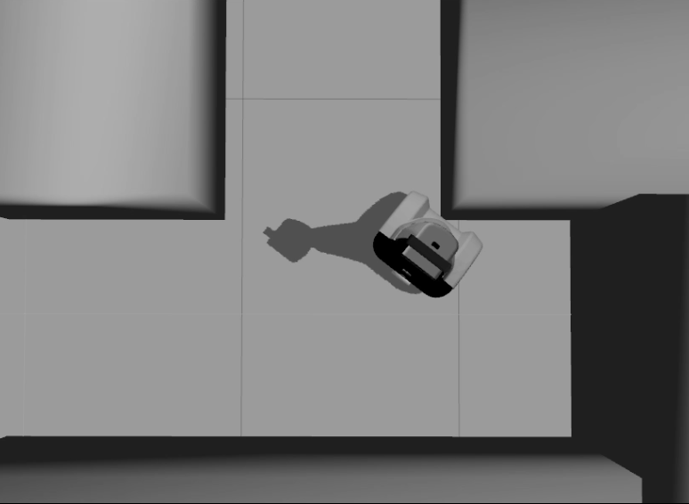
An example of pico recovering is shown in the movie below:

Videos

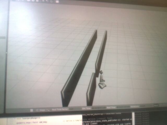
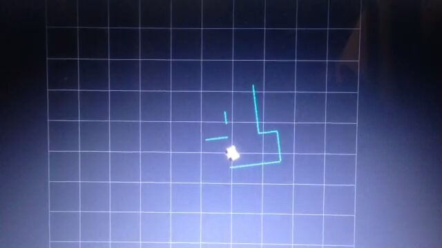
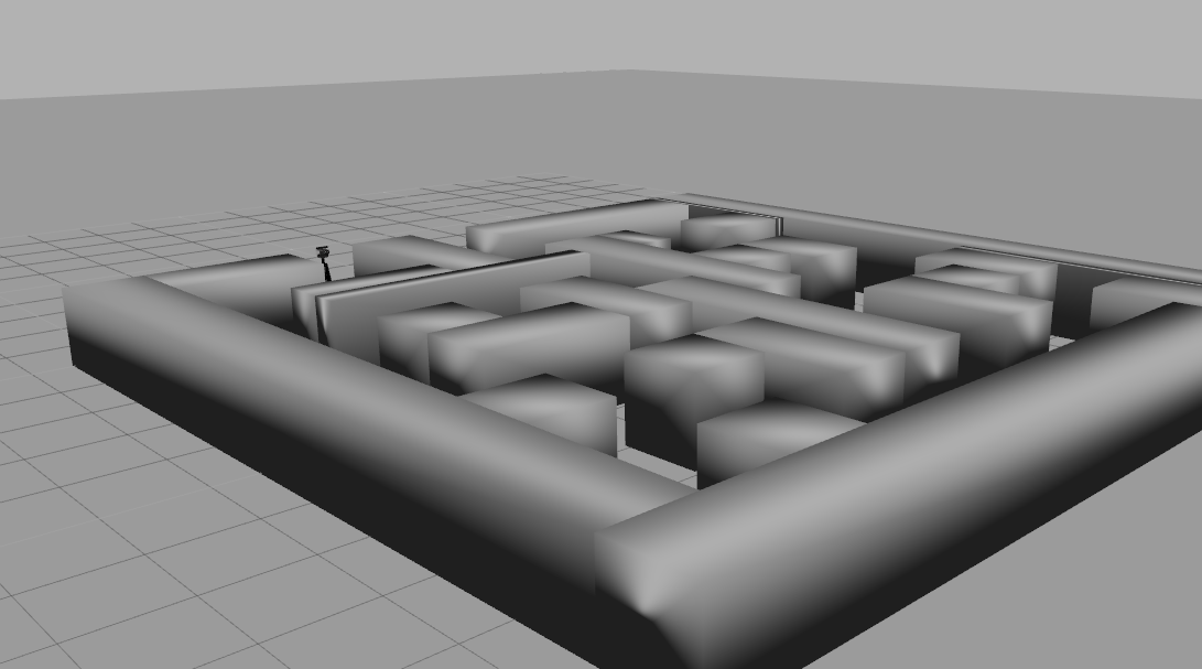
Simulation

Corridor challenge	Line detection	Maze

Real-time

Corridor challenge	Maze
	TBD

References