Embedded Motion Control 2014 Group 1

Group Info

Name:	Student id:	Email:
Groupmembers (email all)
Sander Hoen	0609581	s.j.l.hoen@student.tue.nl
Marc Meijs	0761519	m.j.meijs@student.tue.nl
Wouter van Buul	0675642	w.b.v.buul@student.tue.nl
Richard Treuren	0714998	h.a.treuren@student.tue.nl
Joep van Putten	0588616	b.j.c.v.putten@student.tue.nl
Tutor
Sjoerd van den Dries	n/a	s.v.d.dries@tue.nl

Meetings

Weekly meetings are planned during the course. Every Wednesday a standard meeting is planned to discuss progress with the group and with the tutor. Presentations from these weekly meetings can be found with the presentation links below. Important meeting decisions can be found with use of the meeting liks below. Next to the standard weekly meetings evening meetings are planned to work as a group on the software design.

1. Meeting - 2014-05-02
2. Meeting - 2014-05-12
3. Meeting - 2014-05-14
4. Meeting - 2014-05-15
5. Meeting - 2014-05-16
6. Meeting - 2014-05-21
7. Meeting - 2014-05-23
8. File:Presentatie week 3.pdf
9. File:Presentation week 4.pdf

Time Table

Fill in the time you spend on this course on Dropbox "Time survey 4k450.xlsx"

Planning

Week 1 (2014-04-25 - 2014-05-02)

• Installing Ubuntu 12.04
• Installing ROS
• Following tutorials on C++ and ROS.
• Setup SVN
• Plan a strategy for the corridor challenge

Week 2 (2014-05-03 - 2014-05-09)

• Finishing tutorials
• Interpret laser sensor
• Positioning of PICO

Week 3 (2014-05-10 - 2014-05-16)

• Starting on software components
• Writing dedicated corridor challenge software
• Divided different blocks
  • Line detection - Sander
  • Position (relative distance) - Richard
  • Drive - Marc
  • Situation - Wouter
  • State generator - Joep
• File:Presentatie week 3.pdf

Week 4 (2014-05-17 - 2014-05-25)

• Finalize software structure maze competition
• Start writing software for maze competition
• File:Presentatie week 4.pdf

Week 5 (2014-05-26 - 2014-06-01)

• Start with arrow detection
• Additional tasks
  • Arrow detection - Wouter
  • Update wiki - Sander
  • Increase robustness line detection - Joep
  • Position (relative distance) - Richard
  • Link the different nodes - Marc

Week 6 (2014-06-02 - 2014-06-09)

• Test maze competition software in practice
• Determine bottlenecks for maze competition
• Make system more robust

Corridor challenge

For the corridor challenge a straight forward approach is used which requires minimal software effort to exit the corridor succesfully.

Approach

For PICO the following approach is used to solve the corridor challenge.

• Initialize PICO
• Drive forward with use of feedback control
  • Position [math]\displaystyle{ x }[/math] and angle [math]\displaystyle{ \theta }[/math] are controlled
  • A fixed speed is used, i.e., [math]\displaystyle{ v }[/math]
  • Safety is included by defining a distance from PICO to the wall, where it will stop if the distance becomes [math]\displaystyle{ \lt 0.1 }[/math]m
  • The distance between the left and right wall is calculated. If one of these distances becomes to small PICO will correct to maintain in the middle of the corridor

• If no wall is detected feedforward control is used
  • Drive for [math]\displaystyle{ T_e }[/math] [s] after no wall is detected
• After [math]\displaystyle{ T_e }[/math] [s] PICO rotates +/-90 degrees using the odometry
  • +/- depends on which side the exit is detected
• Drive forward with use of feedback control
• Stop after [math]\displaystyle{ T_f }[/math] [s] when no walls are detected

States PICO corridor challenge

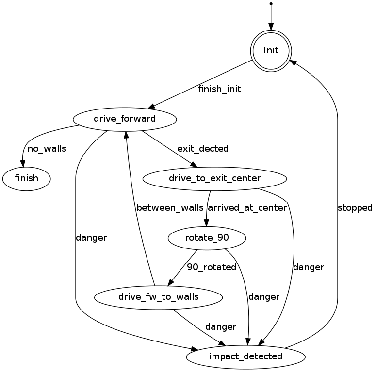
The states of PICO for the corridor challenge are visualized in the following figure:

Result

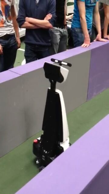
First place!!

Maze challenge

Maze solving algorithm: the wall follower

The choice for this algorithm is based on the fact that its simple, easy to program but nevertheless effective.

Working principle:

This algorithm starts following passages and whenever a junction is reached it always turn right (or left). Equivalent to a human solving a Maze by putting their hand on the right (or left) wall and leaving it there as they walk through.

Examples

Examples of a maze solved by the Wall follower algorithm are shown below.

• Link 1
  
• Link 2
  

Software architecture

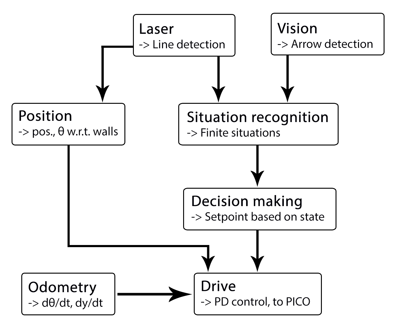THIS FIGURE HAS TO BE ADAPTED!!!

I/O structure

The different components that are visualized in the software architecture scheme are elaborated here

Node	Subscibes topic:	Input	Publishes on topic:	Output	Description
Line detection	/pico/laser	Laser scan data	/pico/lines	Array of detected lines. Each line consists out of a start and an end point (x1,y1),(x2,y2)	Transformation of raw data to lines with use of the Hough-transform. Each element of lines is a line which exists out of two points with a x- y and z-coordinate in the Cartesian coordinate system with Pico being the center e.g. (0,0). The x- and y-axis are meters and the x-axis is the front/back of Pico while the y-axis is left/right.
Arrow detection	/pico/camera	Camera images	/pico/vision	Arrow detected to the left of the right	Detection of arrows pointing to left or right.
Odometry	/pico/odom	Quaternion matrix	/pico/yaw	float with yaw angle	Transform Quaternion in roll, pitch and yaw angles. Only yaw angle is send because roll and pitch are zero.
Distance	/pico/line_detection	Line coordinates	/pico/dist	(y_left, y_right, x, theta_left, theta_right) also known as the 'relative position'	Determine distance to wall to left, right and front wall. Also determines angle left and right with respect to the walls.
Drive	/pico/state /pico/dist	(y_left, y_right, dy, x, dx, theta_left, theta_right,dtheta)	/pico/cmd_vel	Pico moving	Move pico in the desired direction
Situation	/pico/line_detection /pico/laser /pico/vision	Line data, vision interpretation and possibly laser data.	/pico/situation	The situation where pico is in. For example corridor to the right, T-junction, etc.	Situation parameters.
State generator	/pico/situation /pico/yaw	Situation and yaw angle of Pico.	/pico/state	dx,dy, dtheta	Based on the situation Pico needs to go through different states and continue to drive. Every state defines an action that Pico needs to do.

PICO messages

The different nodes are communicating with each other by sending Messages. Each nodes sends a set of messages with use of a publisher. The Message that are sends between the nodes are defined in this section.

Lines

The line message includes two points, p1=(x1,y1) and p2=(x2,y2), which are defined by the geometry messages package. A point consists of (x,y,z) coordinate. For points p1 and p2 the z-coordinate is set to zero.

Points p1 and p2 are connected to represent a line each line is stored in array:

  Line[] lines

The detected lines are visualized as a Marker in rviz, by using the visualization_msgs package.

Situation

Basically, there are eight main situations, these are shown in the figure below. If PICO does not detect any corner points, then it is located in a corridor. In this case the robot can go straight on. If PICO detects any corner points, then it might need to turn. Whether it needs to turn, depends on the situation. The different type of situations are

   Situation T-junction exit left right
   Situation T-junction exit front right
   Situation T-junction exit front left
   Situation Corridor
   Situation Corridor right
   Situation Corridor left
   Situation Intersection
   Situation Dead end

Drive

The drive message sends commands to the drive node which actually sends the velocity commands to pico. The message contains two float32, one to specify the velocity forwards and one to represent the velocity by which Pico turns around his axis.

   float32 speed_angle
   float32 speed_linear

Vision

The vision message contains two booleans for if it either detects an arrow pointing to the left, or a arrow pointing to the right.

   bool arrow_left
   bool arrow_right

I/O principles

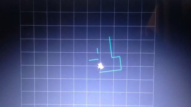
Line detection

Input: "/pico/laser"
Output: "/pico/lines"

Principle

Transformation of raw laser data to lines representing the walls of a corridor. This transformation is done with use of the Hough-Transform

Approach

• Convert laser data to points (x,y,z)
  
  • Transform from sensor_msgs::Laserscan to pcl::PointCloud<T>
• Convert PointCloud to 2d Matrix
  • The 2d matrix represents an 2d image of the scanned area
  • Each detected point is colored white in the 2d image
• Apply hough transform
• Transform lines in image coordinates back to world coordinates
• Filter detected lines
  • Increases robustness by neglectin small gaps within the corridor

Arrow detection

TBD

Relative distance

input topic: /pico/lines
function: Determine distance to wall to left, right and front wall. Also determines angle theta with respect to the corridor.
output: (Y_left, Y_right, X (forward), theta_left, theta_right)
output topic: /pico/dist
msg: dist.msg
float32 YR
float32 YL
float32 THR
float32 THL
float32 X

The angle theta can be calculated with the next fomula:

[math]\displaystyle{ \theta = atan((y2-y1)/(x2-x1)) }[/math]

the position perpendicular to the line/wall is calculated with the next formula:

[math]\displaystyle{ X_r = y2 - ((y2-y1)/(x2/x1))*x2*cos(\theta_1) }[/math]

[math]\displaystyle{ X_l = y4 - ((y4-y3)/(x4/x3))*x4*cos(\theta_2) }[/math]

theta is average of left and right or only left or right depending on situation

Drive

This node sends velocity commands to Pico based on input from the state generator node and relative position node. The state generator node sends a velocity in x and theta based on the state it is in. The relative position node sends the distance and angle relative to the left and right wall with Pico as the centre. When possiblethis information is used for the orientation and positioning of Pico.

Situation

inputs: lines, vision, relative position

Two different approaches are taken into account, a simple approach in which only is detected if the left, front and right side of pico are 'free' of walls/obstacles. But also a more elaborate approach in which situations are detected like, junctions, T-junctions, crossings and dead ends.

Lines can be categorized in two types of lines:
Longitudinal lines: y-coordinates of begin and end point are similar
Lateral lines: x-coordinates of begin and end point are similar

Situations to be recognized:

- inbetween two walls
No obstacles in front, no lateral line detected within X meter.
2 longitudinal lines are detected.

- Junction
3 lines are detected. From which two are longitudinal lines and one is lateral within (X meter).
Detect direction of juction by comparing the x -values of the longitudinal lines with the x-value of the lateral line.
Left junction: When the x value of the left line (the line with the smallest Y values) is 'minimum corridor width' smaller then the x value of the lateral line a gap on the left side is recognized.
Right junction: When the x value of the right line (the line with the smallest Y values) is 'minimum corridor width' smaller then the x value of the lateral line a gap on the left side is recognized.

- Dead end
3 lines are detected. From which two are longitudinal lines and one is lateral within (X meter).
Detect direction of dead end by comparing the x -values of the longitudinal lines with the x-value of the lateral line. When the x values of both longitudinal lines are similar to those of the lateral line a dead end can be recognized.

- T junction: 3 situations named T-right, T-left, T-right-left.
T-right: 3 longitudinal lines are detected, 1 lateral lines detected on the right side of pico.
T-left: 3 longitudinal lines are detected, 1 lateral lines detected on left side of pico.
T-right-left: 2 longitudinal lines are detected: 4 lateral lines are detected

- X junction
4 longitudinal and 4 lateral lines are detected

State generator

input: Situation, relative position
input topic: /pico/sit

function: Create setpoint for position of pico by use of state. (determine wanted position and speed).
output:
output topic: /pico/

msg:

Videos

Simulation

Corridor challenge	Line detection	Maze
		TBD

Real-time

Corridor challenge	Maze
	TBD