Embedded Motion Control 2019 Group 7: Difference between revisions
| Line 514: | Line 514: | ||
<center> | <center> | ||
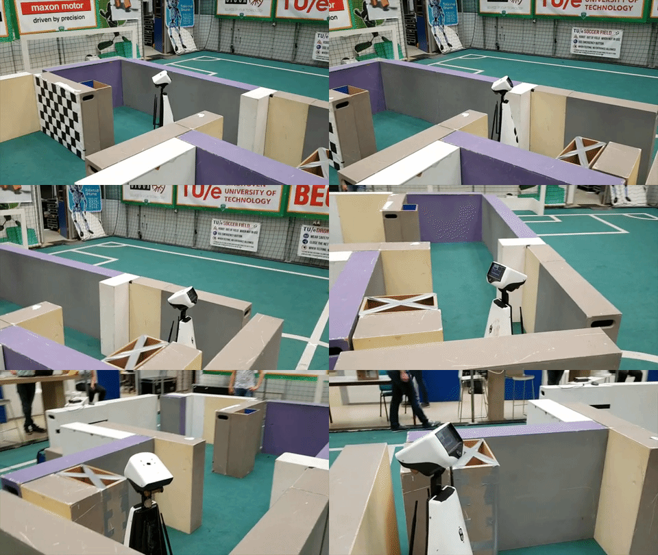
[[File:Group7 2019 Hospital challenge sim with obstacles.gif | center |thumb | [[File:Group7 2019 Hospital challenge sim with obstacles.gif | center |thumb | Part 3 of the final challenge.]] | ||
</center> | </center> | ||
Revision as of 10:58, 21 June 2019
Embedded Motion Control 2019 Group 7: PicoBello
Group members
| Name | Student nr. |
|---|---|
| Guus Bauwens | 0958439 |
| Ruben Beumer | 0967254 |
| Ainse Kokkelmans | 0957735 |
| Johan Kon | 0959920 |
| Koen de Vos | 0955647 |
Introduction
This wiki page describes the design process for the software as applied to the PICO robot within the context of the "Embedded Motion Control" course project. The project is comprised of two challenges: the escape room challenge and the hospital challenge. The goal of the escape room challenge is to exit the room autonomously as fast as possible. The goal of the hospital challenge is to autonomously visit an unknown number of cabinets as fast as possible.
Design Document
The design document, describing the initial design requirements, functions, components, specifications and interfaces, can be found here.
Challenge 1: The escape room
As an intermediate assignment, the PICO robot should autonomously escape a room through a door from any arbitrary initial position as fast as possible.
To complete this goal, the following steps are introduced:
- The sensors and actuator are initialized.
- From the initial position, the surroundings are scanned for gaps between the walls. If no openings are found, the robot is to rotate until the opening is within view.
- The robot will drive sideways towards a subtarget (to prevent loosing the target when moving in front of it), placed at a small distance from the opening in order to avoid wall collisions.
- Once arrived at the subtarget, the robot will rotate towards the target.
- After being aligned with the target, the robot will drive straight trough the corridor.
To this end, methods for the detection of gaps between walls, the placement of (sub)targets and the path planning are required.
Data preprocessing
Beforehand, some of the measured data can already be labelled not useful. That data is summarized below.
- As the provided data structures have built in minimum and maximum values, data that is out of these bounds is first filtered out. This concerns the laser range finder radius and angle.
- Data can have outliers or unexpected readings, therefore data is removed using a low pass filter. Datapoints that have no close by neighboring points are therefore removed.
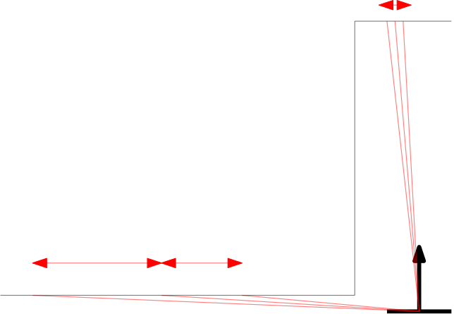
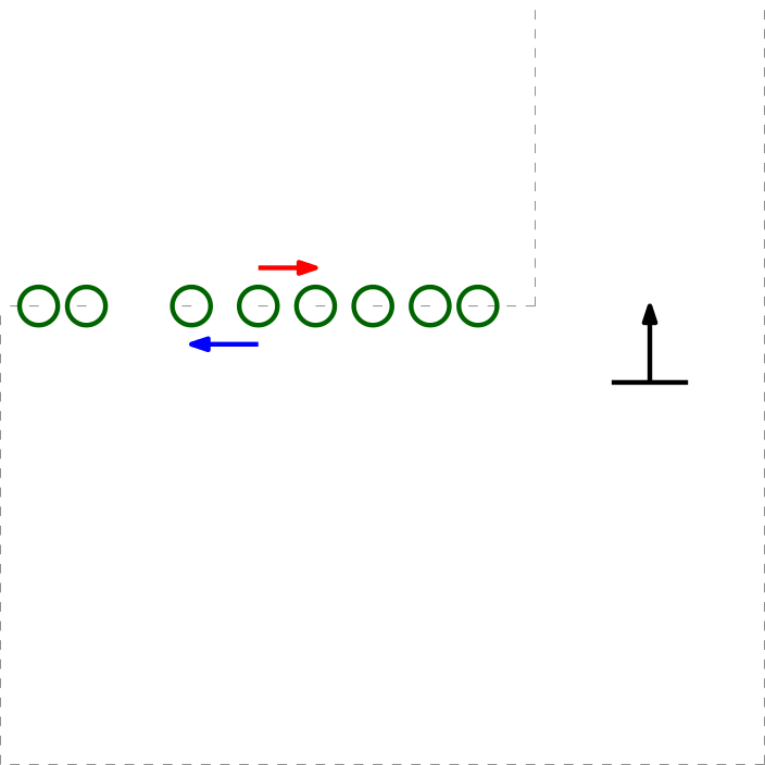
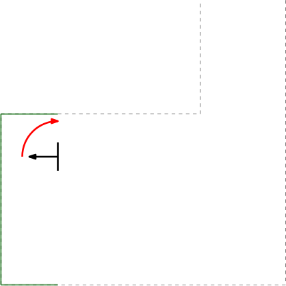
- Next to the initial angle correction, gap detection only works in the range of > 0 and < 180 degrees in front of PICO. This is to prevent reading out data that is perfectly in alignment with PICO's x-axis (lateral direction). This is to prevent data readings as depicted in the left Figure below.
-
Prevent lateral data measuring which cannot be used for gap detection.
-
Remove data that does not have close by points.
Gap detection
From the initial position, the surroundings are scanned using a Laser Range Finder (LRF). A gap is detected when there is a significant jump (of more than 0.4 [m]) between two subsequent data points. This method is chosen for its simplicity, it does not require any mapping or detection memory.
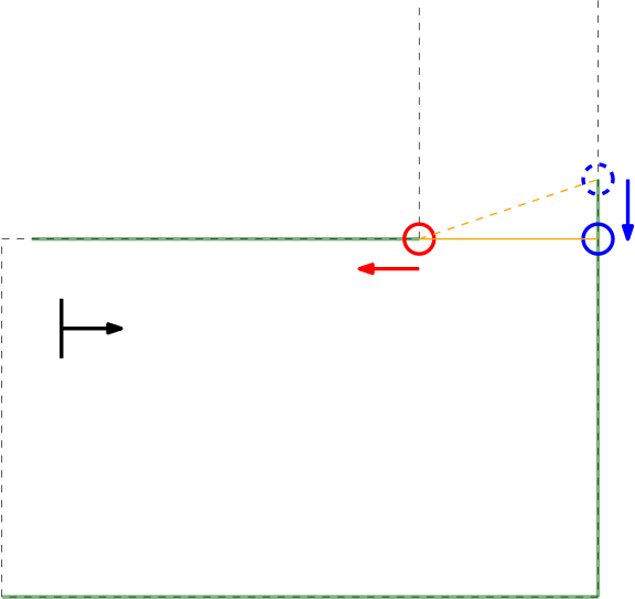
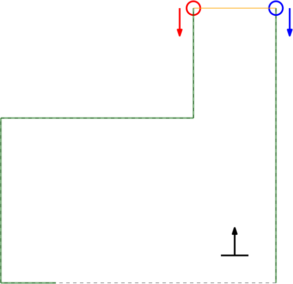
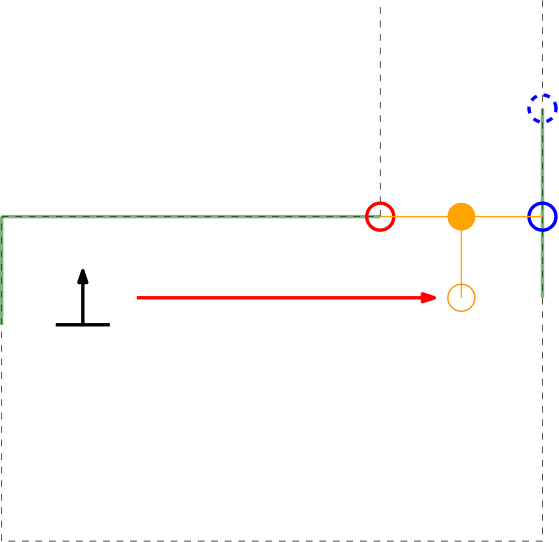
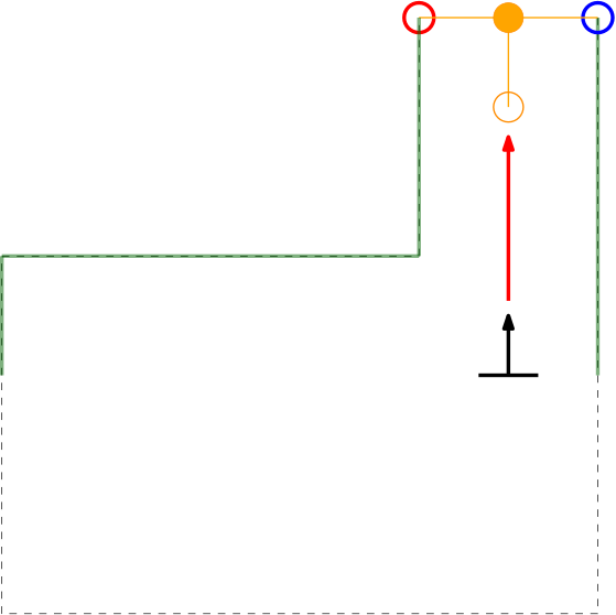
Within the context of the escape room challenge, either from within the escape room or from within the corridor a gap can be detected, as depicted in respectively the left and right Figures below.
As can be seen in these Figures, dependent on PICO's orientation, gaps can be detected under an angle resulting in a sub optimal recognition of the corridor entry. To this end, the gap size is minimized by moving the points on the left and right side of the gap respectively counterclockwise (to the left) and clockwise (to the right). The result of this data processing is shown in the left Figure where the dotted orange line depicts the initial gap, and the straight orange line depicts the final gap. Here, the left (red) point is already optimal and the right (blue) point is optimized.
In the right depicted example of a possible situation, PICO is located straight in front of the corridor. In this case the gap cannot be optimized in the same way because moving either of the points increases the distance between the points (as they are not iterated at the same time). However, the detected gap can be used as target for PICO and should result in a successful exit of the escape room if followed correct.y
-
Scheme of a possible Escape Room, with PICO located in the upper left corner.
-
Scheme of a possible Escape Room, with PICO located in the lower right corner.
Dealing With Boundary Scenarios
Initially 2 detected data points are be expected, 1 of each corner of the exit. This would be the case if the escape rooms exit would have empty space behind it. Topology wise this is true, but in practice the LRF will possibly detect the back wall of the room the escaperoom is placed in or other obstructions standing around the exit.
In the case a (more or less solid) backwall is detected, the gap finder will find 2 gaps, one on each side of the exit. In this case the closest left and right points are taken to set the target. The target is defined as the midpoint between these two closest data points.
(Sub)Target Placement
As driving straight to the target, the midpoint of a detected gap, should actually result in a collision with a wall in most circumstances (refer to the left Figure in the previous section), a subtarget is created. The target is interpolated into the escape room to a fixed distance perpendicular to the gap. This point is first targeted.
PICO will turn on its central axis so that it is facing parallel to the direction of the sub target to the target, and will drive in a straight line to reach it (which is therefore lateral). When PICO is approaching the subtarget, the corridor will become visible. As this removes the discontinuity in the data (as PICO can now see into the corridor), a new target is found consisting out of either 2 or 4 points. In the first case no backwall is detected, in the second case a back wall is detected. In this scenario two gaps will be found; to the left and to the right of the end of the exit. The new target will become the middle of the 1st and 4th point as again the closest left and right point are taken. A subtarget is set, but will not change PICO's desired actuation direction.
Path Planning
The loop of finding gaps is gone through continuously. The following cases are build in:
- 0 data points found
Protocol 1
If no data points are found, PICO should turn until it finds two valid data points which form a gap. If still no data points are found, PICO assumes he is to far away from the exit so switches to protocol 2.
Protocol 2
If after a full turn not data points were found, apparently no gaps are in range. PICO should move forward in a safe direction until it either cannot move anymore, a maximum distance is reached, or data points are detected. If none are detected, return to protocol 1.
- 2 data points found
The 2 points are interpolated as target, the sub target is interpolated. PICO should align itself with the sub target to target direction and move lateral towards it the lateral error is to big. If the lateral error is small enough, move straight forward.
- more than 2 data points found
The closest two points are used to calculate the gap.
-
Step 1 of finding the escape room exit.
-
Step 2 of finding the escape room exit.
-
Step 3 of finding the escape room exit.
Dealing With Discontinuities In Walls
If a wall is not placed perfect, the LRF could find an obstruction behind the wall and indicate it as a gap (as the distance between the escape rooms wall and the obstruction will be bigger than the minimum value of a gap), while in practice the gap is too small to fit through and is not intended as the correct exit. These false positives should be filtered.
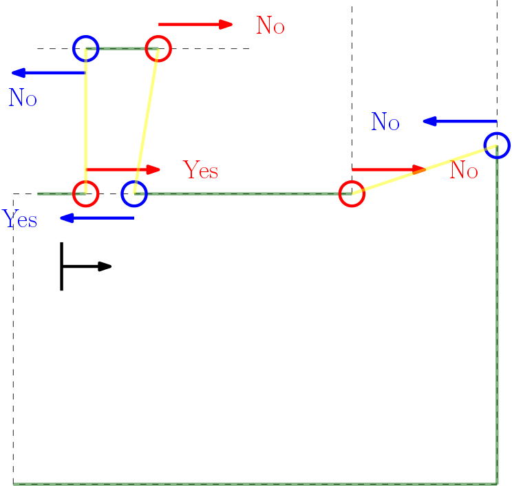
In the Figure below the algorithm used is depicted. From right to left (as this is the direction PICO stores data) first the actual gap is detected (yellow line), then 2 other gaps are detected as the LRF can see through the wall. The first point of every jump (the blue points) are checked for data points to the left that are too close by in local x and y coordinates. If this is the case, the gap cannot be an exit. Likewise, the left (the red points) are checked for data too close by to the right. This is done over all available valid data in the corresponding direction. If data is detected which is too close by, the set of points which form the gap are deleted. Note that the data will not be deleted when a back wall is detected behind the actual exit as the desired gap to be found is big enough.
This detection algorithm will break the exit finding procedure when a back wall is placed to close to the exit, but it is a given that the escape room will have an open exit.
When the algorithm i this to data points found in an actual gap. These points will never be too close by as the blue point will never have a data point to the left closer by then the minimum exit size (as will the red point to the left). Again (correctly) assuming that the escape room has an open exit. Important to note is that this check is done with the initial gap detection data points, not with the optimized location. If it would, in this example the blue point of the actual exit has directly neighboring data to its left (solid blue circle)!
-
Checking discontinuity in walls.
Simulation Validation
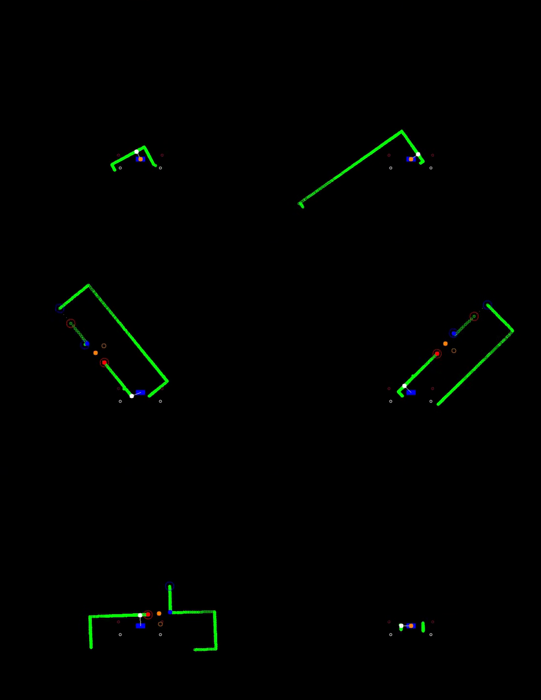
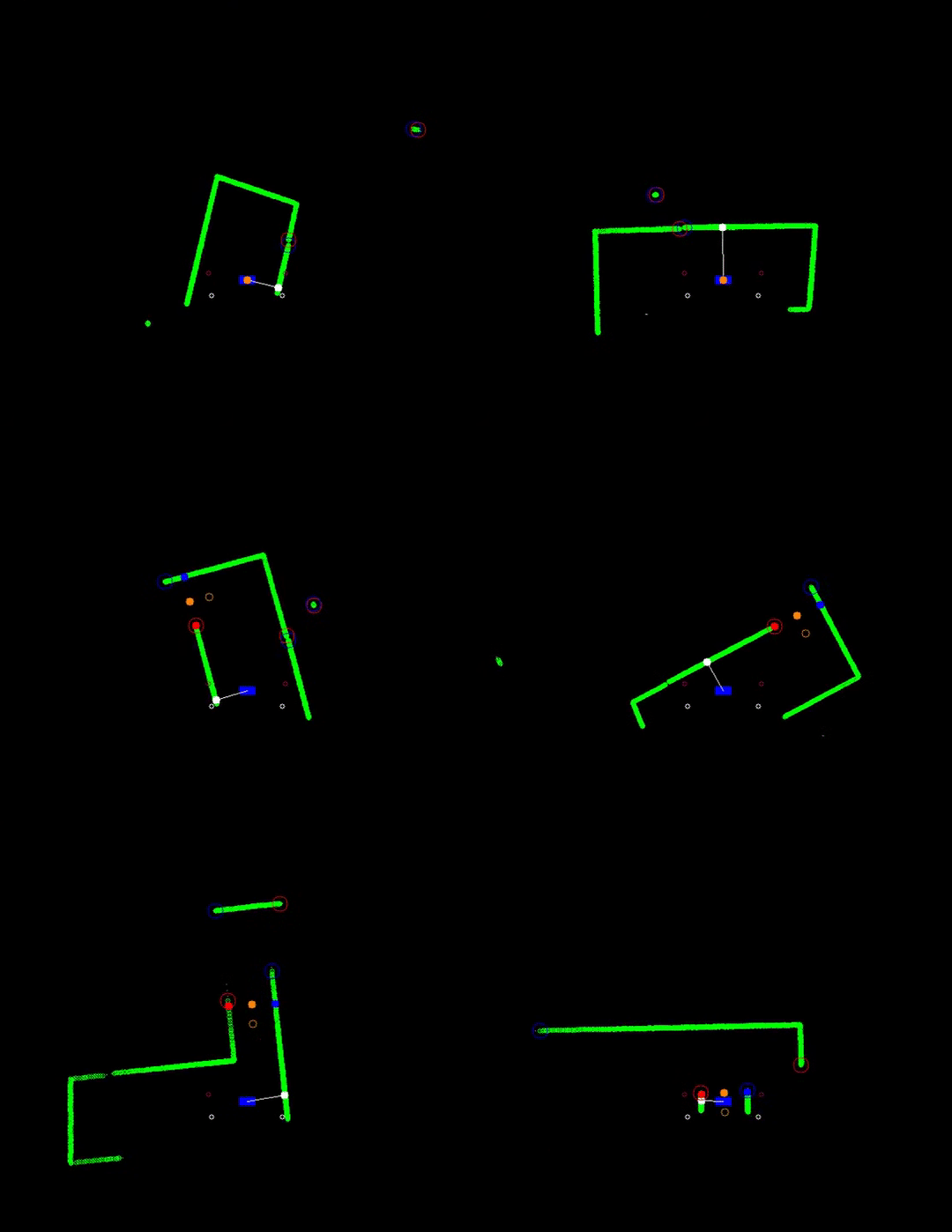
text: TODO morgen
Challenge Review
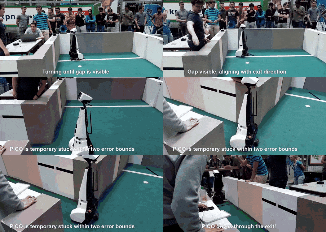
We became second with a finishing time of 60 seconds!
Initially 2 doors where introduced in the escape room. PICO would not have been able to find the correct exit as no check was implemented for the extra requirement that the walls of the exit are 3 m. PICO would have driven to the exit it saw first. If both exits would have been seen at the same time, PICO should have chosen the closest one with a risk of constantly switching between both if the distance is similar. The implementation of first aligning to the direction of the exit would have helped as the other gap should not have been visible anymore.
Despite of completing the challenge successfully, some undesired behavior was observed:
- Due to the long exit walls, PICO kept compensating its orientation position in front of the exit. Buffers which should have limited this behavior where implemented (a valid range for the orientation instead of a single value), but due to the big distance these are currently assumed to be non-sufficient. Also, due to the length of the exit the exit opening was closer to the obstacles around the RoboCup field, which is expected to have partially messed up the non-valid gap detection. Luckily there was a moment where the orientation was correct which moved PICO forwards.
- PICO stopped very close to the finish line. We expect this happened due to too much disturbance behind the escape rooms exit. We always tested with short exit corridors (as explained above), so during the challenge the exit was located much closer to the table standing in the hallway. We expect some other or even no valid exits were seen for a short moment. Luckily PICO did find the valid exit again and drove over the finish line!
- During the first try PICO hit the wall, so the safe distance to a wall should be validated. As we do not have the data, we do not know if the collision was caused by overshoot of the initial driving to sub target or due to not reacting/measuring the wall that was too close. As the second try was programmed to turn to opposite direction for gap detection, we probably avoided this error.
Our lessons learned during the Escape room challenge are that we should:
- be more strict in how we interpreted world information (two exits was technically allowed as one was defined with the correct corridor wall length),
- not assume that certain scenarios (longer walls) work without testing,
- validate the collision avoidance.
Challenge 2: Hospital
Overview
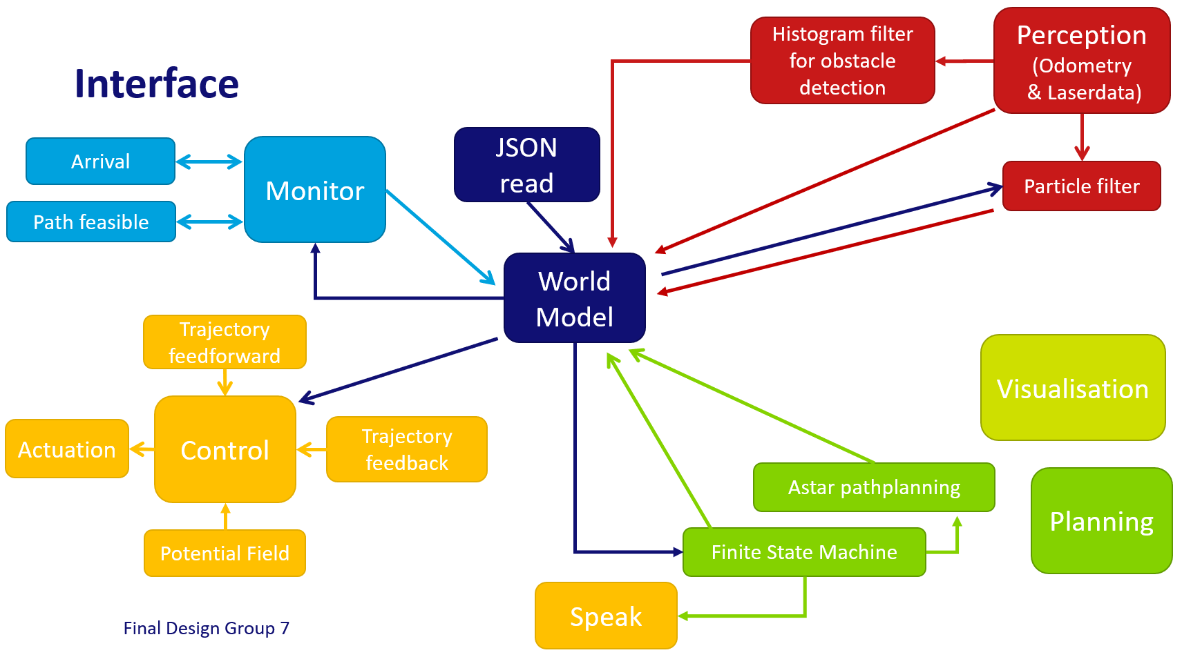
For the hospital challenge, the software design can be split into four parts: Perception, Planning, Monitor and Control. These parts will be explained in the sections below. A schematic overview of the structure and coherence of these components can be seen below. Because it was desired to run several interacting processes at the same time, a software design has been made that can cope with this. The implementation of this design is shortly explained in the section Implementation.
Perception
The perception component is responsible for translating the output of the sensors, i.e. odometry data and LRF data, into conclusions on the position and enivorment of PICO.
Localization on the global map is performed using a particle filter. Detection of static obstacles is done using a histogram filter.
Monte Carlo Particle Filter (MCPF)
In the hosptial challenge it is very important that PICO is able to localize itself on the global map, which is provided before the start of the challenge. The particle filter is responsible for finding the starting location of PICO when the executable is started. After the initilization procedure it will keep monitoring and updating the position of PICO based on the available LRF and odometry data.
General Implementation
Initialization
When the excecutable is started PICO does not know where it is, besides being somewhere in the predefined starting area. In order to find the most likely starting position (more on this later), an initialization procedure was devised which is able to, whithin a limited time frame, find a set of possible starting positions. Finding this starting position is best described by the following pseudo code.
...
loop for N times
{
Intialize particles randomly
Calculate probability of particles
Pick and store X particles with largest probability
}
...
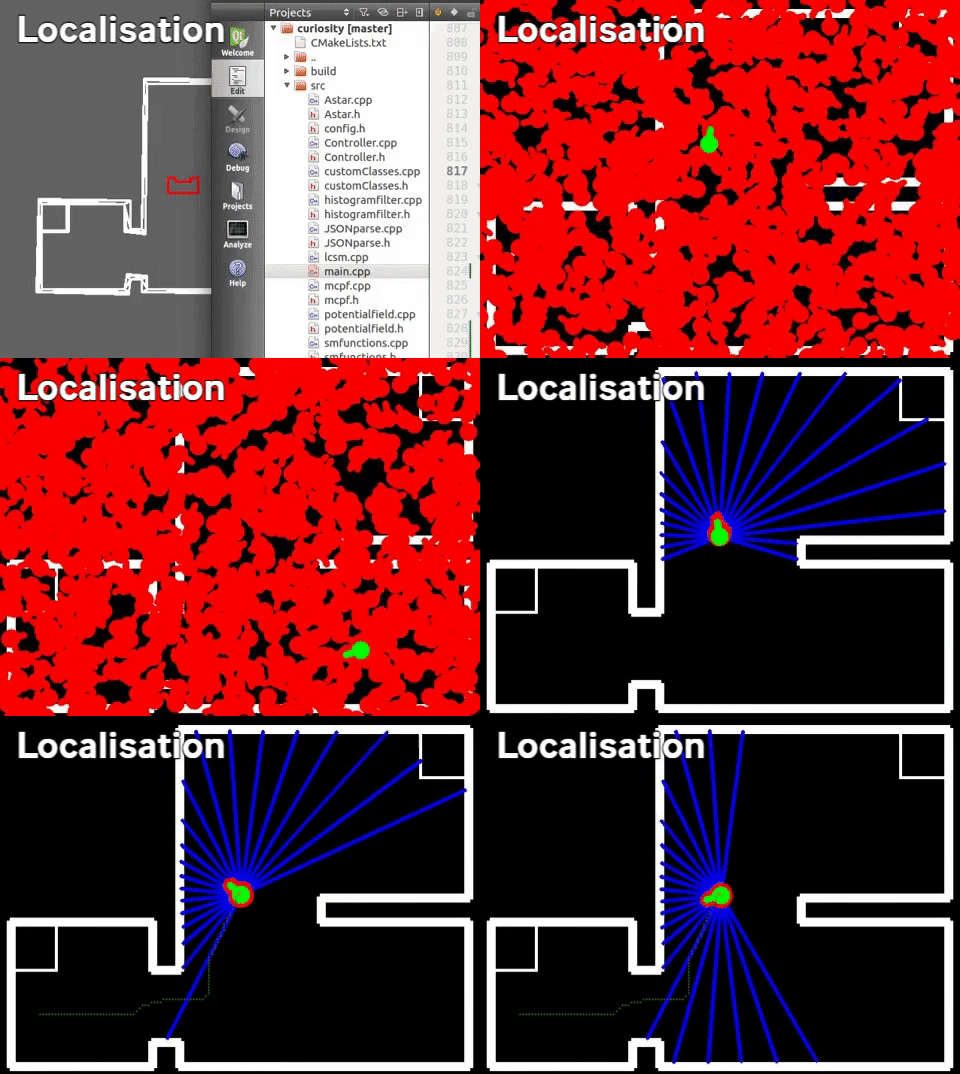
This algorithm provides the particle filter with a list of particles which describe the possible starting position of PICO. This list of particles is then used as an initial guess of the probability distribution which describes the location of PICO. This distribution is not necessarily unimodal, i.e. it is possible that a certain starting position delivers identical data with respect to another starting location. It is therefore not possible to immediately conclude that the mean of this distribution is the starting location of PICO. The probability distribution stored in the particle filter must first converge to a certain location, before the mean position can be send to the world model. Convergence of the probability distribution is tested by calculating the maximum distance between "likely" particles, in which a "likely" particle is defined as a particle with a probability larger than a certain value. This distance is constantly monitored to determine whether convergance has been achieved.
Often it is not possible for the particle filter to converge without additional information. This is for instance the case when PICO is in a corner of a perfectly square room with no exit and perfectly straight corners. In this case the particle filter will first signal to the state machine that it has not yet converged, the state machine will then conclude that it has to start turning or exploring to provide the particle filter with extra information on the current location of PICO. When sufficient information has been collected to result in an unique location and orientation for PICO the particle filter will signal the state machine that it has converged. After convergence the particle filter will start its nominal operation, described below.
Propagating on the basis of odometry data
After initialization of the particle filter the starting position of PICO is known, however PICO is a mobile robot so its position is not constant. It is possible to run the initialization procedure every iteration to find the new location of PICO, this is however not very efficient. We know the probability distribution of the location of PICO in the last iteration, before it moved to a new location. Additionally we have an estimate of the difference in location since we last calculated the location of PICO, this estimate is namely based on the odometry data of the wheel encoders of PICO. This estimate can be used to propagate all particles, and thereby propagate the probability distribution itself, to the new location.
In simulation this propagating of the particles on the basis of the wheel encoders would exactly match the actual difference in location of PICO, as there is no noise or slip implemented in the simulator. In reality these effects do occur though. In order to deal with these effects a random value is added to the propagation of each particle. This makes sure that the particles are located in a larger area than would be the case if the particles were propagated naively, without any noise. This larger spread of particles then ensures that the actual change of location of PICO is still within the cloud of particles, which would not be the case when the spread of particles was smaller. The amount of noise that is injected in propagating the particles is a fraction of the maximum allowed speed of PICO, in the final implementation this fraction is set to 10 percent.
In pseudo code the propagating of particles can be described in the following way:
...
for all particles
{
X = sample(uniform distribution (a,b))
Y = sample(uniform distribution (a,b))
O = sample(uniform distribution (c,d))

x location  += xshift + X
y location  += yshift + Y
orientation += oshift + O
}
...
Find probability of each particle
Up until now the described particle filter is only able to create and propagate particles, however it is not yet able to conclude anything about its current position in any quantitative way. A probability model for each particle is needed before any conclusions can be drawn. The LRF data is the perfect candidate to draw conclusions on the current position of PICO. The LRF data does not have the disadvantage of the odometry data, i.e. that it is unreliable over large distances. The LRF data by definition always describes what can be seen from a certain location. It is possible that there are objects within sight, which are not present on the map, however it will later be shown that a particle filter is robust against these deviations from the ideal situation.
The probability of a particle is defined on the basis of an expected measured LRF distance and the actually measured distance. This however assumes that the expected measured LRF distance is already known. This is partly true, as the approximate map and particle location are both known. Calculating the distance between one point, given an orientation and map, is however not a computationally trivial problem. In order to efficiently implement the particle filter, given the time constraints of the EMC course, it was chosen to use a C++ library, to solve the so called raycasting problem. The documentation, github repository, and accompanying publication of the range_libc library can be found in the references. [1] In order to be able to run the particle filter in real time the fastest algorithm, i.e. Ray Marching, was chosen to be used in the particle filter. The exact working of these raycasting algorithms will not be discussed on this wiki.
With both the measured and expected distance (based on the particle location) known, it is possible to define a probability density function (PDF), which maps these two values to a likelihood of the considered ray. In this implementation the decision was made to choose a PDF which is combination of a uniform and gaussian distribution.[2] The gaussian distribution is centered around the measured value and has a small enough variance to drastically lower the likelihood of particles that do not describe the measurement, but a large enough variance to deal with noise and small mapping inaccuracies. The uniform distribution is added to prevent measurements of obstacles immediately resulting in a zero likelihood ray. The likelihood of rays is assumed to be independent, this is done in order to be able to easily calculate the likelihood of a particle. When the measurements are independent the likelihood of a particle is namely the product of the likelihoods of the rays. After determining the likelihood of each particle, their likelihoods need to be normalized such that the sum of all likelihoods is equal to one.
In order to implement the above stated probability model two important deviations from this general setup were made. Firstly it was noticed that it is difficult to represent the particle likelihoods, before normalization, using the standard C++ data types. Given that the above stated probability model has a maximum value of approximately 0.6, it is easy to compute that even likely particles, which each contain 1000 rays, will have likelihoods smaller than 1e-200. In order to solve this problem another way of storing the likelihoods was devised. For the final implementation a scientific notation object was developed. In this object two values are stored separately. A double to store the coefficient and an integer to store the exponent. This allows us to store a large range of very small and very large values.
A second implementational aspect has to do with the maximum achievable execution speed. One can imagine that the before stated raycasting algorithm is quite heavy to run, compared to other parts of the software. In order to prevent slow downs the particle filter is assigned a separate thread, as discussed before. However to further reduce the execution time a decision was made to down sample the available data. Out of all 1000 available rays, only 100 are used. There is a risk of missing features when heavy down sampling is used, however no significant reduction in accuracy has been noticed due to down sampling the available data. In literature, most notably the source of the ray casting library, down sampling the LRF is standard practice in order to reduce the computational load.[3]
Finding Location of PICO
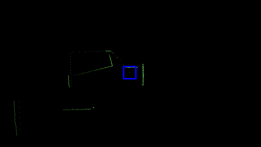
With the probability distribution (represented by the particles and their likelihoods) known, it is possible to estimate the location of PICO. Ideally one would take the geometric median of the probability distribution to find the most likely position of PICO. However taking the median of a three dimensional probability distribution is not trivial. One could take the median over each dimension, however this is not guaranteed to result in a location which is actually in the distribution. The initialization procedure was devised in order to tackle this problem. The procedure makes sure that the distribution is unimodal. Given this unimodal distribution it is possible to take the weighted mean of the distribution to find the most likely location of PICO.
Resampling
The "real trick" [2] and important step of the particle filter algorithm is re-sampling. A particle filter without re-sampling would require a lot more particles in order to accurately describe the earlier discussed probability distribution. This hypothetical particle filter would have a lot of particles in regions where the likelihood is very small. The basic idea of re-sampling is to remove these particles from the particle filter and replace them either with a random particle, or with a particle placed in a region with a high probability. Selection of particles is done in a non-determenisitic way, a particle is chosen with a probability of its likelihood.
In re-sampling it is often preferred to also inject random particles in the filter. Random particles allow the particle filter to re-converge to the true location when the current estimate is no longer valid. The risk of random particles is most apparent in an identical room situation. A particle that is initialized in a situation close to identical to the true location will lead to a risk of losing the true estimate. In this implementation random particles are not injected into the filter during normal operation, to prevent losing the accuracy of the estimate.Since it is expected that the location of PICO is always within reasonable range of the estimated position, it is not necessary to inject random particles.
Resampling is done using a resampling wheel.[4]A re-sampling wheel is an algorithm which allows us to re-sample the particles in the particle filter without having to make and search a list of the cumulative sum of all likelihoods, which would be required when one would draw a random number and select a particle purely based on the interval in which this number is located. Our implementation of the re-sampling wheel can be found in the code snippet at the end of this page. Conceptually a re-sampling wheel works in the following way. Some changes to the maximum step size were made in order to incorporate random particles and dynamic resizing of the amount of particles in the particle filter.
Obstacle Detection
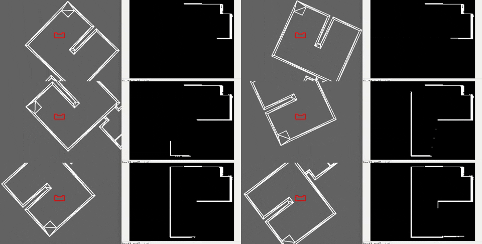
The perception of PICO is not limited to finding its position on the provided map. Based on the location data, provided by the MCPF, PICO is able to keep track of obstacles and walls that it can see using its LRF. Based on this observations it creates a secondary map using the histogram filter described in this chapter. A Histogram filter is a well known method in literature to keep track of obstacles. [2]
General Implementation
The histogram filter contains a grid map of the probabilities of objects in a certain location. This grid map is initialized at robot start up as an uniform distribution. When one ray of PICO lands inside an element of this grid, i.e. when PICO detects something in this grid square, the histogram filter will update the likelihood of an object at this location. Updating the likelihood is done according to Bayes theorem, which effectivley means that the probability is incrementally updated at each observation. The big advantage of this approach is that multiple observations of an object are necessary before conclusions are drawn. The incremental updating decreases the sensitivity of the histogram filter for noise on the observations, outliers in the data and most importantly (sufficiently) dynamic objects. It is expected that dynamic objects change location every few seconds. Obstacles who do not meet this requirement are classified as static objects, for as long as the object is at that location.
Not only does detecting an object provide information about the presence of an object, so does not detecting an object at a certain location (negative information). This is for instance the case when we know that a certain detection is only possible when there is no object between PICO's current location and the object that was detected. In order to test whether this is the case for points in the grid a point polygon test is performed, using OPENCV. The polygon is defined as the cloud of LRF data around PICO, the points that are inside this polygon provide information on the absence of objects.
In order to be less sensitive for mapping inaccuracies it is important to realize that only local information can be fully trusted. A slightly shorter corridor could otherwise be recognized as an obstacle when viewed from a distance. Therefore a maximum range is set which can be updated. When a point is outside of this range, in the final implementation two meters, it will not be updated. This does not only make the implementation more robust it also significantly decreases the required computational time.
Furthermore to prevent path infeasibilities, and therefore increase robustness, it is explicitly assumed that all cabinets are reachable. When the path planning algorithm becomes infeasible the histogram filter is re-initialized as a uniform distribution. This removes all detected objects from the map, making the path feasible again. Due to the specifics of the implementation this will only remove the objects, the original provided map will remain known to the robot and path planner.This might not be the most elegant solution, when the path is infeasible PICO would ideally start exploring to discover where objects are not located, however due to the time limit of the project this could not be implemented.
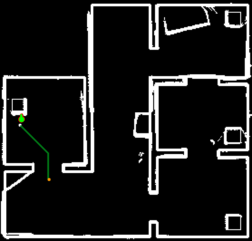
Performance
The performance of the localization, performed by the particle filter, and obstacle detection, performed by the histogram filter, is best analyzed simultaneously. Inaccurate estimates provided by the particle filter would be an input of the histogram filter, and would therefore immediately be noticeable on the obstacle map. It can furthermore be checked whether the histogram filter is robust enough to the slight variations in estimates of the location provided by the particle filter.
In various test sessions the particle filter was able to find and keep the correct location in various situations. The first situation includes mapping inaccuracies, such as wall which are up to 0.5 meter shorter than expected and walls which are rotated approximately 10 degrees. Secondly obstacles which are not on the map do not result in the particle filter losing its localization, these obstacles can be quite large as shown in the hospital challenge. During tests PICO also drove into a bag and enclosed in thight spaces, which did not result in losing its location.
The output of the particle and histogram filters after completing the final hospital challenge are shown in the Figure next to this chapter. The output shows the estimated position of PICO in green and the particles in the particle filter in red. The obstacles and walls are plotted in white and part of the path of PICO is shown as a green line. It can be seen that all of the objects that were added to the hospital environment during the challenge are present in the output of the perception. It should be noted that only the front of these objects are present, since this is the only part of the objects that is actually visible.
Some of the objects present in the output can not be explained as being a static object. The first of which are the diagonal lines which are present next to cabinets. The origin of these points is explained when one views the LRF data of PICO. When sharp corners are encountered it is possible that the LRF returns on the lines shown in the output, this is due to the inner working of the sensor. Normally these points are removed after some time due to the working of the histogram filter, however this is not the case in the area around cabinets. This is because PICO will hardly see this area, without being in front of the cabinet. The histogram filter does not have the time to see that there is no object there.
The second non static object seen on the output are some seemingly random groups of pixels located, among other, next to the boxes in the corridor. This can likely be explained when one watches the video of the final challenge. The dynamic object stands still for some time next to these boxes. The histogram filter likely recognizes this as an object, and afterwards does not have to chance to see that there is actually no object there.
World Model
Our world model lays at the basis of our coding structure. Using an adapted version of the provided JSON parser, the JSON map is converted to a .png which can be used by the software. Furthermore, as the rules of which is the front of a cabinet are known (the first line in a cabinet), the cabinet targets are set automatically. This software structure allows to run in principle all possible (valid) maps automatically. Nothing is hard-coded based on specific characteristics of a map.
Due to an unknown cause it is however necessary to run the code twice to correctly load a new JSON file as writing the new file is not completed before the file is done writing. The old file is loaded in when this happens.
The world model handles the pose of PICO with its global x, y and angle. Furthermore the histogram filter updates a copy of the map to be used in the A* algorithm to avoid measured obstacles. If for some reason no path can be found the histogram map is cleared.
State machine
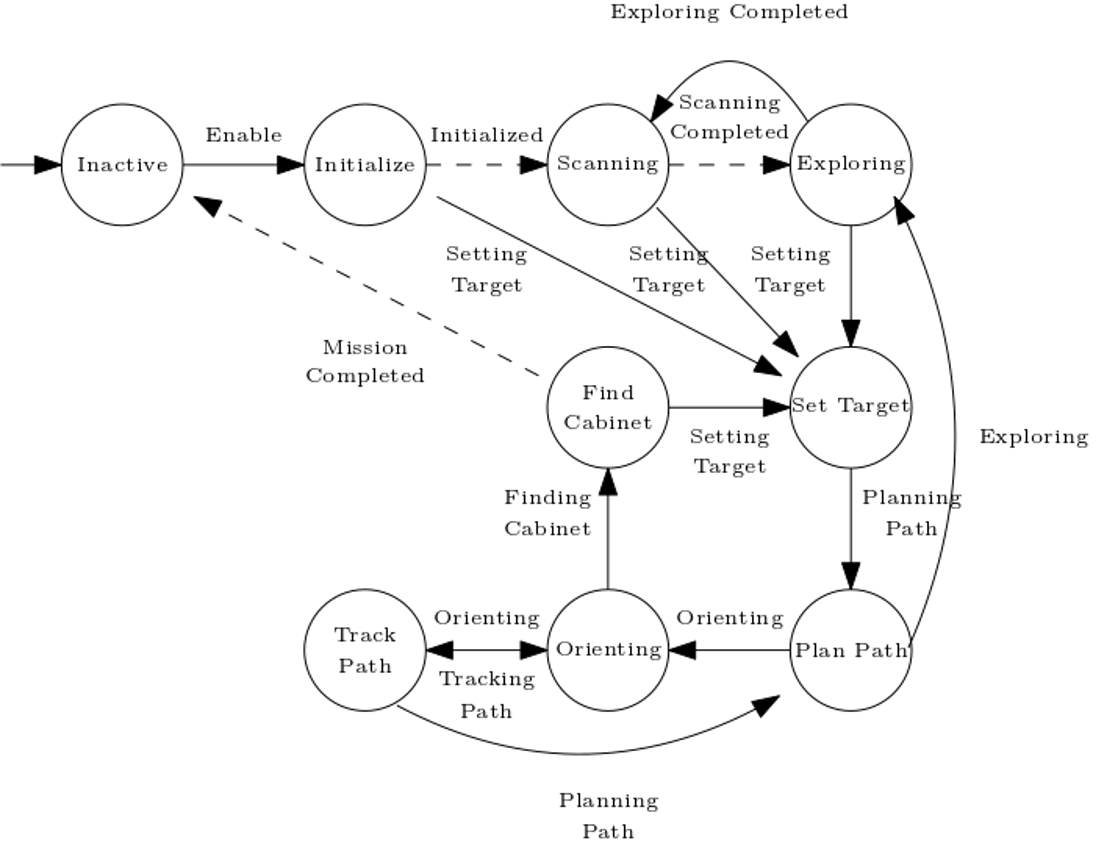
A finite state machine is designed as a means of sequential control logic, which forms the core of the system’s architecture. It allows for traversing through a predetermined sequence of states in an orderly fashion, facilitating the coordination of activities and behaviors. A total of nine behaviors are implemented, as depicted by the circles in the schematic overview of the state machine in the figure below. The basic operation within each state is twofold: (1) running the output function, which generates the state machine output, and (2) running the transition function, which generates the value of the next states dependent on the value of the state’s guards. Below, a quick overview of the functions of each of the implemented behaviors is provided.
Inactive
This is the initial and resting state of the robot. The robot enters it to wait for new instructions after finishing its tasks.
Initializing
While the particle filter is initializing, the robot will remain in the initializing state. As movement is of no added value in this state, the robot will stand still until the initialization is finished. Generally, this state is traversed through quite quickly.
Scanning
Once the particle filter is initialized, the aim is for the particle filter to convergence as fast as possible. To this end, a scanning algorithm is in place as it is minimally invasive to its surroundings and yields a lot of information. During this procedure, the robot turns on its axis for a little over ??? degrees, allowing for a 360-degree map of its surroundings. During scanning, the robot will warn its environment about its turning movement using a speak command. The frequency at which speak commands can be sent is limited to avoid saying multiple sentences at the same time. In addition, the last sentence pronounced is kept track off, to avoid sentence repetition.
Exploring
If scanning the entire surroundings is not sufficient for the particle filter to converge, PICO will be ordered to drive around to explore its surroundings. The robot will drive in the direction of doors and open spaces, by moving towards the furthest measured LRF distance point. The potential fields are activated during all movement, including exploring, to prevent collisions. Out of safety precautions, the total driving distance is limited to just half a meter. Once this distance is completed, the robot return to the scanning state to map the surroundings on its new position in a 360-degree fashion. A big advantage of this implementation is that it allows proper localization even within similar looking rooms. Often, driving just a small distance towards the door gives sufficient insight for the particle filter to properly converge. In addition to the localization procedure, the exploring state forms part of the path planning procedure. The algorithm comes in play when no path to the destination can be found. This usually implies that some object, be it static or dynamics, is blocking. First, the static object map is cleared. Then, the robot will enter an exploring-scanning loop, until a path is found to the destination. This procedure prevents deadlock, even in the case of unreachable goals and is a vital backup plan in the software as not making sensible movements for 30 seconds can call for a disqualification. In addition, being able to move around is time efficient, as allows for further static obstacle mapping while waiting for a path to the destination to be found. During exploring, the robot will warn its environment about its movement using a speak command as well.
Setting target
This state is in charge of determining which target the robot should go to next. In this state, the targets are clipped using an up-to-date static object map. This prevents target placement on locations that are impossible to reach, e.g. targets too close to the wall or static objects. The target will be clipped within the defined cabinet region as close as possible to the “ideal” target, which is placed at a standard distance in front of the center of the cabinet.
Planning path
In this state, a path is planned towards the current target using an A* algorithm. During operation, the robot will reach this state in three cases: (1) a new target cabinet is set and requires the first path, (2) the orientation or position of the robot deviates too far from the planned trajectory, or (3) new static obstacles are detected on the current path. The replanning frequency is limited to a tenth of the sampling frequency, to prevent deadlock issues due to infinite looping between the path planning and orienting states when there are multiple slightly deviating possible paths.
Tracking path
In the tracking path state, the ‘normal’ control strategy using feedforward and feedback, will steer the robot towards its desired trajectory and orientation. The robot will warn its environment about its movement using a speak command, and state the target cabinet number.
Orienting
A separate state is implemented for orienting without driving. This state is activated in two cases: (1) if the orientation of the robot deviates too far from the planned trajectory, or (2) when the robot has arrived at a cabinet and needs to orient to face it straight on. This prevents driving in directions outside of laser range finder view.
Finding a cabinet
Once the robot has reached its target, its finding cabinet procedure is twofold: (1) a speak instruction is sent to the robot, mentioning at which cabinet it has arrived, and (2) a snapshot of the laser data will be saved in the group folder.
Monitor
The monitors, within the context of this project, are the Booleans that allow for discrete perception of the system dynamics. The monitors act as the state’s guards, which implies that their involvement in the state machine is twofold: (1) guards trigger state transitions dependent on their current value, and (2) guards are updated as a consequence of each state transition execution. A total of 24 monitors are used in the software. A few examples of these monitors are Booleans indicating that the MCPF is converged, that the scanning is complete or that an obstacle is detected on the current path.
Planning
Path planning with A*
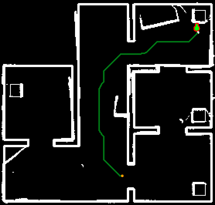
The basic A* search algorithm implementation in C++ was taken from [5] with L2/Euclidean distance heuristic. It was then altered to suit our needs:
- It was adjusted to be able to work with Open CV matrices and to return a path as a stack of integer nodes in the matrix instead of only printing it.
- The map provided by the histogram filter was adjusted such that
- The walls of the provided map were thickened (Open CV convolve with kernel of robot size) to not plan through areas which PICO cannot reach due to its dimensions.
- The areas at the current target and current position are opened up to prevent planning problems when driving close to a wall (or stray pixel from the histogram filter).
- The cost to come g[n] was originally the cost to come of its parent g[n-1] summed with the distance from the node to its parent (i.e. 1 or 0.5[math]\displaystyle{ \sqrt{2} }[/math]). This cost to come has been summed with a non-linear function of the distance to the closest pixel (so after thickening the walls) according to (in a similar fashion to the potential fields): [math]\displaystyle{ g }[/math][[math]\displaystyle{ n }[/math]] = [math]\displaystyle{ g }[/math][[math]\displaystyle{ n }[/math]-[math]\displaystyle{ 1 }[/math]]+[math]\displaystyle{ \alpha }[/math][math]\displaystyle{ x }[/math]-[math]\displaystyle{ n }[/math], in which [math]\displaystyle{ \alpha }[/math] and [math]\displaystyle{ n }[/math] can be tuned to put to paths closer or further away from the walls. As seen in the snapshot on the right, the planned path passes through the middle of corridors as opposed to the regular A* algorithm that will cut create as close to the walls as possible to minimize the traversed distance.
Trajectory reconstruction
Once the path is generated by A*, it should be converted to a trajectory, i.e. a time varying reference that can actually be tracked by the controller. The following pseudo-code specifies how the path is converted to a trajectory:
Compute the maximum distance d_max that can be traversed in the given sample time based on the given velocity limits
Set trajectory at current time to current position
Set current node to first node of A* path
while the path is not traversed
{
    while selected node is not in reach of current position with d_max
    {
        Increment current position with d_max into the direction of the selected node
        Append incremented position to the trajectory
        Append corresponding velocity to velocity trajectory
    }
    while current node is in reach of current position with d_max
    {
        Loop over path until node is found that is out of reach given d_max
        Set current node to found node
        Calculate direction from current position to next node using atan2
    }
}
Return trajectory and velocity trajectory
Like this, a path is interpolated between the nodes found by A*. Sufficiently low sampling times have been chosen in combination with margins from the wall in A* such that interpolation will never result in a trajectory that comes too close to a wall. The calculated velocity can be used as feedforward in the controller, which results in perfect tracking without feedback in simulation, validating the trajectory and velocity reconstruction.
Control
When PICO knows its current pose (location and orientation) and its desired pose or trajectory, the software should determine which velocities (translational and rotational) will be sent to the base to achieve this in a stable and safe way. The chosen control strategy consists of two main parts:
- A 'normal' control strategy using feedforward and feedback to steer PICO towards its desired pose or trajectory, based on the world model.
- An extra check to avoid bumping into walls and (static and dynamic) obstacles by steering PICO away from those when it comes to close, based on the direct LRF data.
On a semantic level, these two strategies interact as follows: when PICO is not so close to walls and obstacles, the normal control strategy will dominate. When PICO comes very close to a wall or obstacle, the extra check will start to have more and more influence, to prevent bumping into them, even when the normal controller would steer PICO into their direction. The two seperate strategies are explained in more detail in the subsections below.
Normal control strategy
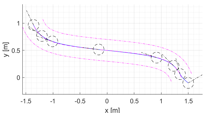
The controller is designed such that it 1) exploits PICO’s holonomicity when driving small distances close to walls and 2) ensures that PICO drives forward when driving for longer distances through big corridors. This is realized by
- converting the planned path in global coordinates and global pose estimate to global position errors,
- mapping the global positions errors into the local frame, resulting in a local x and y error,
- applying a linear feedback law on these local errors, implemented as a simple gain as the plant can be modeled as an integrator,
- while simultaneously controlling the orientation into the direction of the path.
This local mapping ensures that PICO is controlled in both local x and y, while the rotation controller ensures that the error is directed in x solely in the local x coordinate given that there is enough time to get to the orientation reference. Like this, PICO starts driving holonomically when the orientation error is large and gradually converges to driving forward when the orientation error is reduced. A deadzone was included on both the local position errors as well as the orientation. This deadzone was complemented with a feedforward based on the velocities as calculated in the path conversion. The deadzone and the feedforward together form a kind of guarded motion: open loop inputs are applied until PICO deviates too much from its prescribed path.
Obstacle avoidance
The need of an extra safety check
Once the path has been planned and is tracked by the feedforward and/or feedback controller, there still is a risk to hit a wall or obstacle. The most important factor of this risk are dynamic obstacles, which are not coped with on a semantic level anywhere else in our code. Another part of this risk is caused by the fact that the path is planned based on the (updated) map and the tracking is done by means of the pose estimation from the particle filter. However, this pose estimation can and will have a small error, an obstacle could somehow not have been included in our (updated) map, etcetera. Therefore, a more direct approach is used as an extra safety means to avoid obstacles locally: potential fields.
Working principle
The potential fields are based on only the most recent LRF data. In a small neighborhood (a square of 2 by 2 meter) around PICO, a local gridmap is made, with dots (the LRF data) that indicate where walls/obstacles are. This map is then converted to a field, in which the height is an indication of the distance from that point to its closest wall/obstacle. The scaled (discretized) gradient of this field is used as the actuation for the translational directions of PICO, to prevent collisions.
Using only the direct LRF data for these potential fields also has a disadvantage: there is no data available in the region behind PICO. This problem is to a large extent overcome by not driving backwards.
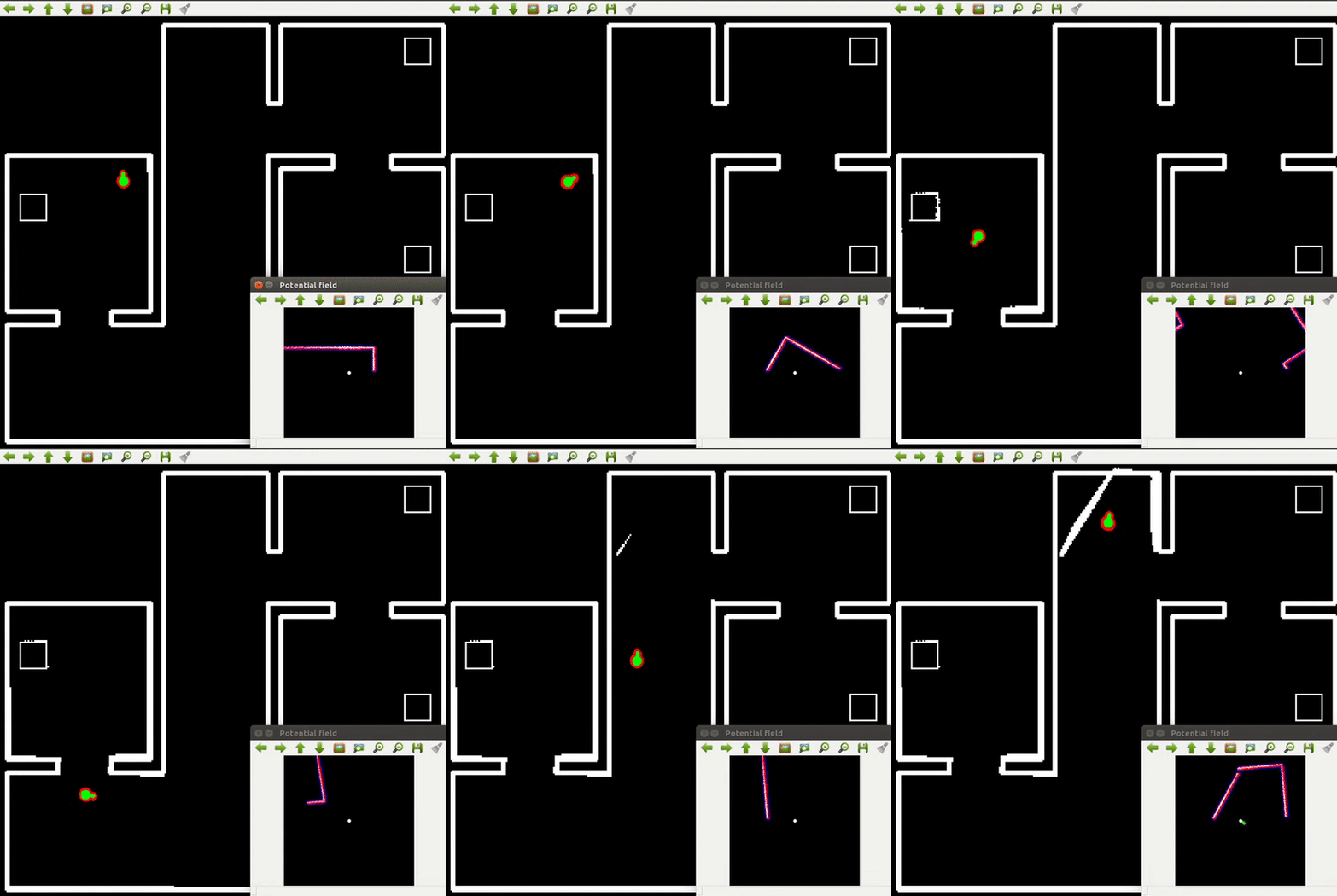
Mathematical implementation
For the resolution of the local gridmap, a balance has been found between accuracy and speed by choosing 120 pixels per meter, giving an accuracy of slightly less than a centimeter. Such an accuracy is required, because PICO should be pushed away from obstacles and walls when they are very close, but the potential fields should not push PICO away too early, because then PICO would for example not be able to drive through a small gap. Given that the width of PICO is about 40 cm and it is desired to still be able drive through a gap of about 50 cm, the potential fields should thus not totally counteract the controller anymore at a distance of about 5 cm from a wall. Taking a too small distance is dangerous, because PICO will not always drive through gaps perfectly straight and the robot is not round but rather square with rounded edges. When simulating and testing, taking 3.5 cm appeared to be a suited value.
The minimum size PICO should be able to drive through, quite a tight fit!
Further, it is not desired that there is a specific distance from obstacles that causes the potential fields to switch from providing no force to full force. Therefore, the slope of the field should increase gradually when coming closer to the wall. This has been implemented by shaping the field with the function:
[math]\displaystyle{ f(x) }[/math] = [math]\displaystyle{ \alpha }[/math][math]\displaystyle{ x }[/math]-[math]\displaystyle{ n }[/math]
in which [math]\displaystyle{ f(x) }[/math] is the height of the grid point in the field, [math]\displaystyle{ \alpha }[/math] is a constant that will be explained later, [math]\displaystyle{ x }[/math] is the distance from the grid point to its closest grid point with an obstacle and [math]\displaystyle{ n }[/math] is the tunable exponent that determines to fast the function decreases for increasing [math]\displaystyle{ x }[/math]. Dividing by zero is avoided by first taking the maximum of x and a very small distance [math]\displaystyle{ x }[/math][math]\displaystyle{ m }[/math][math]\displaystyle{ i }[/math][math]\displaystyle{ n }[/math] = 1 cm. The (negative) gradient* of this field will be added to the reference that is sent to the base. When there would for example only be a wall in front of PICO, we can consider the one dimensional case, in which the gradient is the derivative:
[math]\displaystyle{ d }[/math][math]\displaystyle{ f(x) }[/math]/[math]\displaystyle{ dx }[/math] = -[math]\displaystyle{ n }[/math][math]\displaystyle{ \alpha }[/math][math]\displaystyle{ x }[/math]-[math]\displaystyle{ n }[/math]-[math]\displaystyle{ 1 }[/math]
*The gradient has in fact been implemented as the finite central difference in both directions. When choosing the grid size small enough and the exponent [math]\displaystyle{ n }[/math] not too high, this low order approximation will remain valid. The 'flattened' field (due to taking the maximum of [math]\displaystyle{ x }[/math] and [math]\displaystyle{ x }[/math][math]\displaystyle{ m }[/math][math]\displaystyle{ i }[/math][math]\displaystyle{ n }[/math]) also will not cause any problems, as before the LRF would ever observe a 'wall' at 1 cm distance, PICO would already have made a horrible crash.
Instead of using [math]\displaystyle{ \alpha }[/math] and [math]\displaystyle{ n }[/math], it would be desirable to have a distance [math]\displaystyle{ d }[/math] and the exponent [math]\displaystyle{ n }[/math] as tuning knobs. If the distance [math]\displaystyle{ d }[/math] should be the distance at which the potential fields always cause full actuation away from the obstacles, independent of the normal controller, it should hold that:
[math]\displaystyle{ n }[/math][math]\displaystyle{ \alpha }[/math][math]\displaystyle{ d }[/math]-[math]\displaystyle{ n }[/math]-[math]\displaystyle{ 1 }[/math] = [math]\displaystyle{ 2 }[/math][math]\displaystyle{ v_{max} }[/math]
in which [math]\displaystyle{ v_{max} }[/math] is the maximum velocity, which is also used to bound the normal controller output. Using two times this velocity therefore ensures that full actuation in the opposite direction can be achieved. Rewriting the formula above yields:
[math]\displaystyle{ \alpha }[/math] = [math]\displaystyle{ 2 }[/math][math]\displaystyle{ v_{max} }[/math][math]\displaystyle{ d }[/math][math]\displaystyle{ n }[/math]+1/[math]\displaystyle{ n }[/math]
which has been implemented in the software, so that the tuning knobs are [math]\displaystyle{ d }[/math] and [math]\displaystyle{ n }[/math]. As explained above, a suited value for [math]\displaystyle{ d }[/math] was found to be 23.5 cm (half the robot width plus the margin of 3.5 cm). A suited value for [math]\displaystyle{ n }[/math] partly depends on the used normal controller (due to the interaction with it as explained above), and was in our case found to be about 2.5.
Implementation
To implement the multiple components described above in one design for the software, several approaches could be used. A simple approach would be to loop over all components, every time in the same order. However, some components need more time for one iteration than other components, and for some components a high update rate is not even necessary. For instance, the potential fields are based on the LRF data, which is updated at 40 Hz, so updating the potential fields at a higher rate would not increase the performance. Further, an advantage of separating some components from the main code, is that it makes the code more structured. Therefore, it has been decided to use multi-threading, using POSIX Threads[6]. Since the working of the different components has already been explained in detail in the sections above, what each thread contains is only discussed very globally here.
The different threads
- In the main function, first the initialization is done, in which also the other threads are created. After that, the main function enters the main loop, which contains the state machine and sends the desired reference velocities to the base.
- A separate thread is used to run the particle filter and the histogram filter. This thread uses the map and updates it with the found obstacles. Based on this map, an estimate of the pose is calculated.
- Another thread uses the LRF data to calculate the potential field and the resulting desired (extra) actuation.
- The last thread provides the visualization. It takes the most recent matrices for the images available and shows them all on the screen.
Communication between threads
The important data is shared using a mutex ('mutually exclusive'), which prevents that a variable would be read and/or written at two places in the code at the same time. To prevent that different threads have to wait for each other as much as possible, they are only used to write the local value of a variable to the global one, or vice versa. These local variables can then be used in the rest of the code of each thread, without using a mutex. For example, for the pose estimate of PICO, there is a global variable, a local vairable in the particle filter thread and a local variable in the main thread (for the state machine). The particle filter in general uses its local variable to update the estimate, but after each iteration, it will set the global variable equal to its local variable. The main loop uses its own local variable everywhere in the state machine, but updates it from the global variable at the start of every iteration.
Summary
In summary, a robotic control software has been designed and implemented as an integrated part of the autonomous robot PICO. The software is split into four components: Perception, Planning, Monitor and Control, all linked by a world model. For Perception, a Monte Carlo Particle Filter (MCPF) and a histogram filter are implemented to respectively localize on the global map and detect of static obstacles. For Planning, a state machine is designed to facilitate the coordination of the different implemented behaviors, and an A* algorithm is used for the path planning. For Monitor, a total of 24 monitors have been implemented which are used to trigger transitions in the state machine. For Control, a feedforward and feedback controller is implemented to steer towards the desired trajectory. Potential fields interfere with this signal, to avoid bumping into obstacles.
Final Challenge
As a general overview of the course of the challenge, a few gifs of the challenge attempts in both real life and in simulation with commentary are presented.
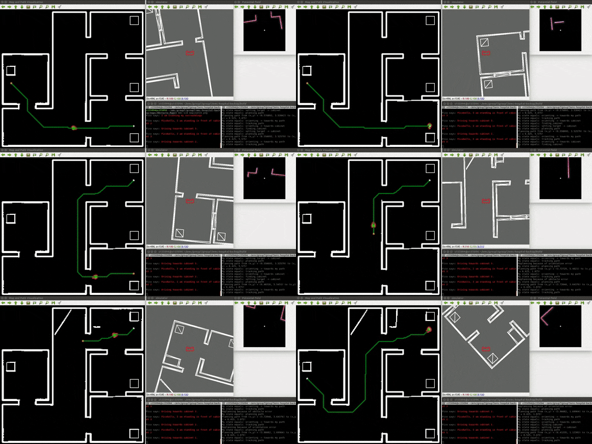
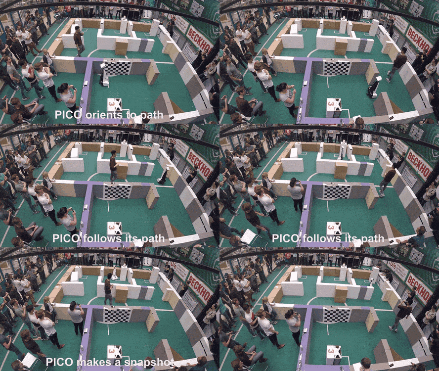
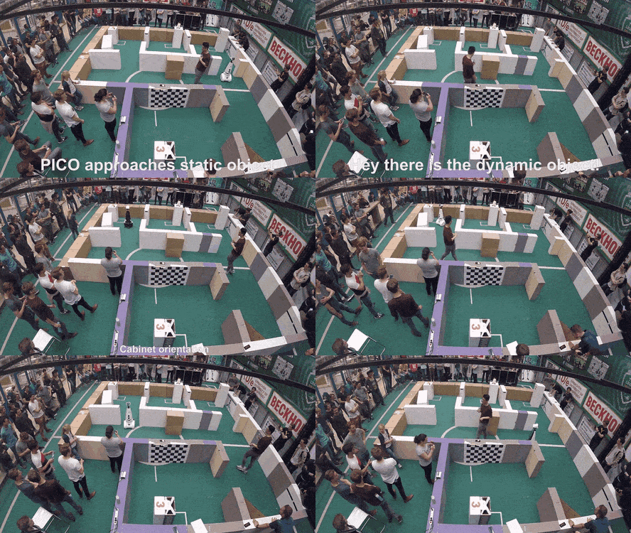
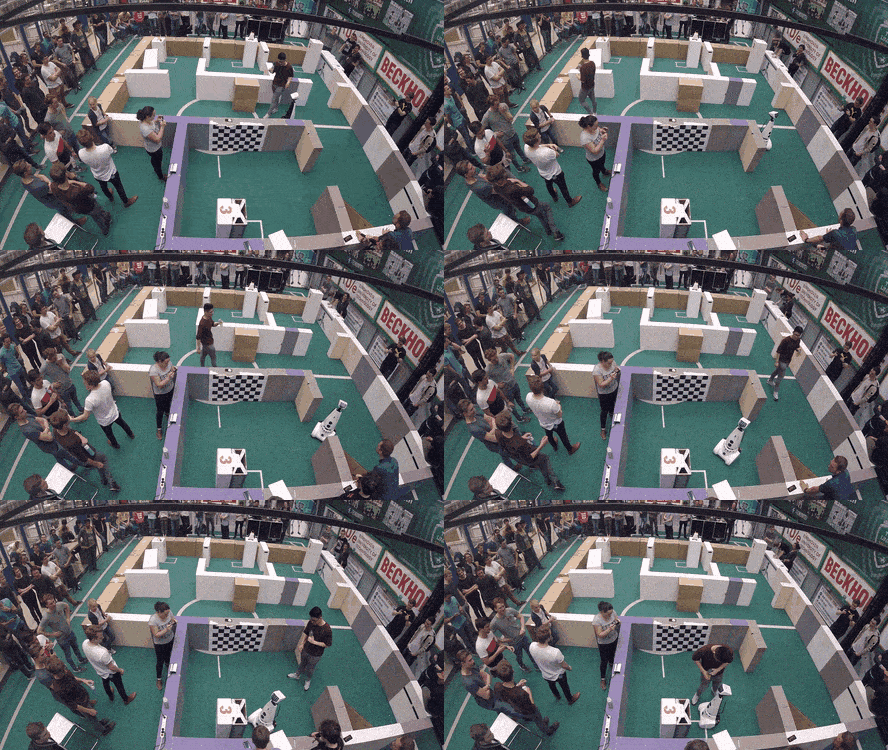
In general, the Hospital Challenge went quite well. We became first with a finishing time of 2 minutes and 26 seconds. All four software components worked well individually. The MCPF converged really quickly and localization was retained at all times. The histogram filter showed proper mapping of the static obstacles and the potential fields demonstrated appropriate (static and dynamic) obstacle avoidance.
During the challenge, only one issue occurred, which was spotted in the testing session the day before. Due to four software components that where individually but not collaboratively tuned, the robot often stood either too close, too far away, or badly oriented in front of the cabinet. This concerned: (1) the potential fields, (2) the target clipping, (3) the cabinet reached monitor, and (4) the output function for the finding cabinet state. This problem could have been solved by proper tuning of the component settings in a real life environment. However, as no additional testing time was available, the tuning was performed in simulation.
During the challenge, this resulted in two unwanted behaviors in front of the cabinets. Although the distance to the cabinet was now by far not as largely varying, it seemed too short on average. This caused the robot to even bump into one cabinet. In addition, the angular restraint on the cabinet reached monitor seemed to tight, which implied that the robot needed a little push before continuing its path to the new cabinet.
Luckily, as we were well aware of the risks of large software changes without testing, we held a backup of our software back in case this would happen. The backup ran quite smoothly and completed the hospital challenge without any issues, other than standing too far in front of the cabinet, as expected.
Snippets
Resampling Wheel[1]
Overall structure and class defenition of MCPF [2]
References
Credits to Group 1 2019 for the wiki layout
- ↑ kctess5(2017). range_libc: A collection of optimized ray cast methods for 2D occupancy grids including the CDDT algorithm. Written in C++ and CUDA with Python wrappers. https://github.com/kctess5/range_libc
- ↑ 2.0 2.1 2.2 [p.125] Thrun, S., Burgard, W., & Fox, D. (2006). Probabilistic robotics. Cambridge, Mass: The MIT Press.
- ↑ H. Walsh, Corey & Karaman, Sertac. (2018). CDDT: Fast Approximate 2D Ray Casting for Accelerated Localization. 1-8. 10.1109/ICRA.2018.8460743.
- ↑ Resampling Wheel - Artificial Intelligence for Robotics : https://youtu.be/wNQVo6uOgYA
- ↑ A* Search Algorithm in C++. Retrieved at: https://www.geeksforgeeks.org/a-search-algorithm/
- ↑ The Open Group Base Specifications Issue 7, 2018 edition: http://pubs.opengroup.org/onlinepubs/9699919799/basedefs/pthread.h.html
