Integration Project Systems and Control 2013 Group 3: Difference between revisions
| Line 239: | Line 239: | ||
{| | {| | ||
|- | |- | ||
| ''' | | '''Trajectory generation''' | ||
|- | |- | ||
| | | The trajectory was built with the LSBP path generator. The trajectory was structured in such a way that LSBP function could at any moment be changed with the quintic polynomial path generator. The trajectory was built using the the shortest possible path. The lowest pizza will be transported to the lowest position, the middle pizza to the middle position and the highest pizza to the highest position. The lowest pizza will be first transported, then the middle and then the highest pizza. The robot arm will move from point to point (see figure below), moving only in one direction at a time, except when rotating without pizza. It will also change height during that motion.<br/> | ||
|- | |- | ||
|} | |||
<br/> | |||
{| | {| | ||
| '''Reference points for trajectory''' | |||
|- | |||
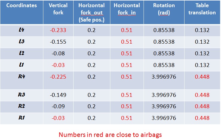
| The following reference points have been taken to be used in the trajectory profiles (these references are based on the images of week1): | |||
{| | |||
|[[File:Group3_References.jpg|thumb|500px|]] | |||
|} | |} | ||
|- | |||
|} | |} | ||
<br/> | <br/> | ||
| Line 268: | Line 276: | ||
| [[File:Axis4FRF.jpg|Axis4FRF.jpg|thumb|400px|]] | | [[File:Axis4FRF.jpg|Axis4FRF.jpg|thumb|400px|]] | ||
|} | |} | ||
|- | |- | ||
Revision as of 21:26, 2 June 2013
Group Members
| Name: | Student id: | Email: |
| Joep Alleleijn | 0760626 | j.h.h.m.alleleijn@student.tue.nl |
| E. Romero Sahagun | 0827538 | e.romero.sahagun@student.tue.nl |
| M. Kabacinski | 0789360 | m.j.kabacinski@student.tue.nl |
| N. Kontaras | 0827208 | n.kontaras@student.tue.nl |
| A. Simon | 0676675 | a.s.simon@student.tue.nl |
Planning
| Week: | Activities: | |
|---|---|---|
| Feb 18 - Feb 24 | ||
| - Make a list for the requirements of the controller | ||
| - Prepare and conduct tests for coupling/decoupling(JA,NK,MK) 3.5 hours | ||
| - Prepare and conduct tests for non linearity (JA,NK,MK) 3.5 hours | ||
| - Prepare and conduct tests for joint identification and create FRF models of the joints (JA,NK,MK) 5 hours | ||
| - Set up DH transfer matrices (AS) 5 hours | ||
| - Generate Matlab Simulation of the kinematic chain (ER) 7 Hours | ||
| Feb 25 - Mar 3 | ||
| - Finish tests for moving direction and create FRF models of the moving direction, moving direction is (JA,NK,MK) 5 hours | ||
| - Design PID feedback controller, add feedforward and test on the robot for each axis of freedom (JA,NK,MK) 11 hours | ||
| - Prepare testing procedure, for following of the trajectory and checking of the requirements (JA,NK,MK) 1.5 hours | ||
| - Matlab code for trajectory generation (TG) (ER) 5 hours | ||
| Mar 4 - Mar 11 | ||
| - Test controllers on the robot (JA,NK,MK) 2 hours | ||
| - Test trajectory generation on the simulation (ER) 3 hours | ||
| - Integrate Inverse Kinematics with Controllers (AS,ER) 2 hours | ||
| Mar 12 - Mar 19 | ||
| - Consider different controller design methods (JA,NK,MK,AS,ER) 10 hours | ||
| - Work on report (JA,NK,MK,AS,ER) 2 hours | ||
| Mar 20 - Mar 27 | ||
| - Test routine generation on the robot (JA,NK,MK,AS,ER) 2 hours | ||
| - Select optimal routine (JA,NK,MK,AS,ER) 4 hours | ||
| - Problem solving (JA,NK,MK,AS,ER) 10 hours | ||
| - Consider different controller design methods (JA,NK,MK,AS,ER) 10 hours | ||
| - Test different controllers (JA,NK,MK,AS,ER) 5 hours | ||
| - Work on report (JA,NK,MK,AS,ER) 2 hours | ||
| Mar 28 - Apr 4 | ||
| - Work on report (JA,NK,MK,AS,ER) 15 hours | ||
| - Prepare presentation (JA,NK,MK,AS,ER) 5 hours |
Progress
Week 1: Feb 18 - Feb 24
 |
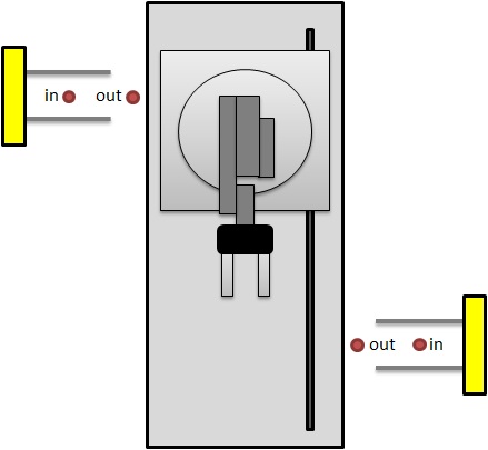 |
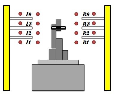
From these images it was decided to program the movement of the pizzas in the following order: L2->R2->L3->R3->L4->R4, using the "out" position of these references as safe position. L1 and R1 are used as well as safe positions.
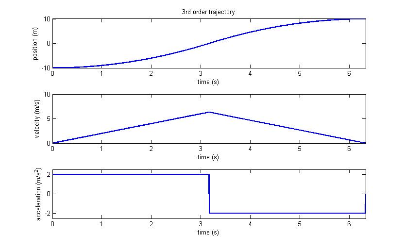
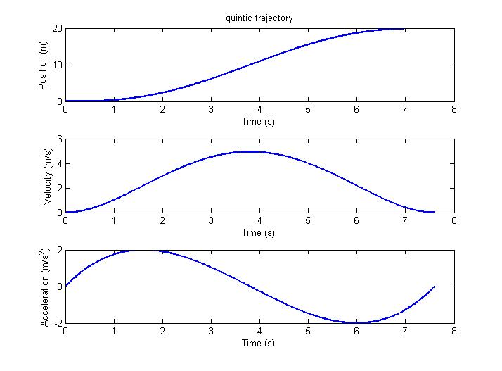
Third order (constant acceleration) and Quintic polynomial trajectory functions have been programmed, as well as a generic script for path generation using these functions. The functions allow to create the fastest trajectory between two points based on acceleration restrictions.The typical position, velocity and acceleration profiles generated by these functions are plotted below.
|
|
Week 2: Feb 25 - Mar 3
| Trajectory generation |
| The trajectory was built with the LSBP path generator. The trajectory was structured in such a way that LSBP function could at any moment be changed with the quintic polynomial path generator. The trajectory was built using the the shortest possible path. The lowest pizza will be transported to the lowest position, the middle pizza to the middle position and the highest pizza to the highest position. The lowest pizza will be first transported, then the middle and then the highest pizza. The robot arm will move from point to point (see figure below), moving only in one direction at a time, except when rotating without pizza. It will also change height during that motion. |
| Reference points for trajectory | |
The following reference points have been taken to be used in the trajectory profiles (these references are based on the images of week1):
|
| Open loop FRF measurement |
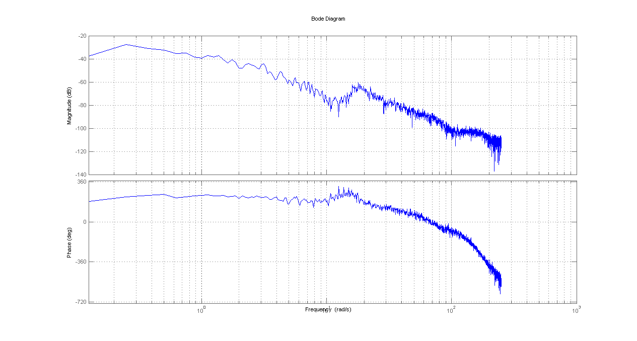
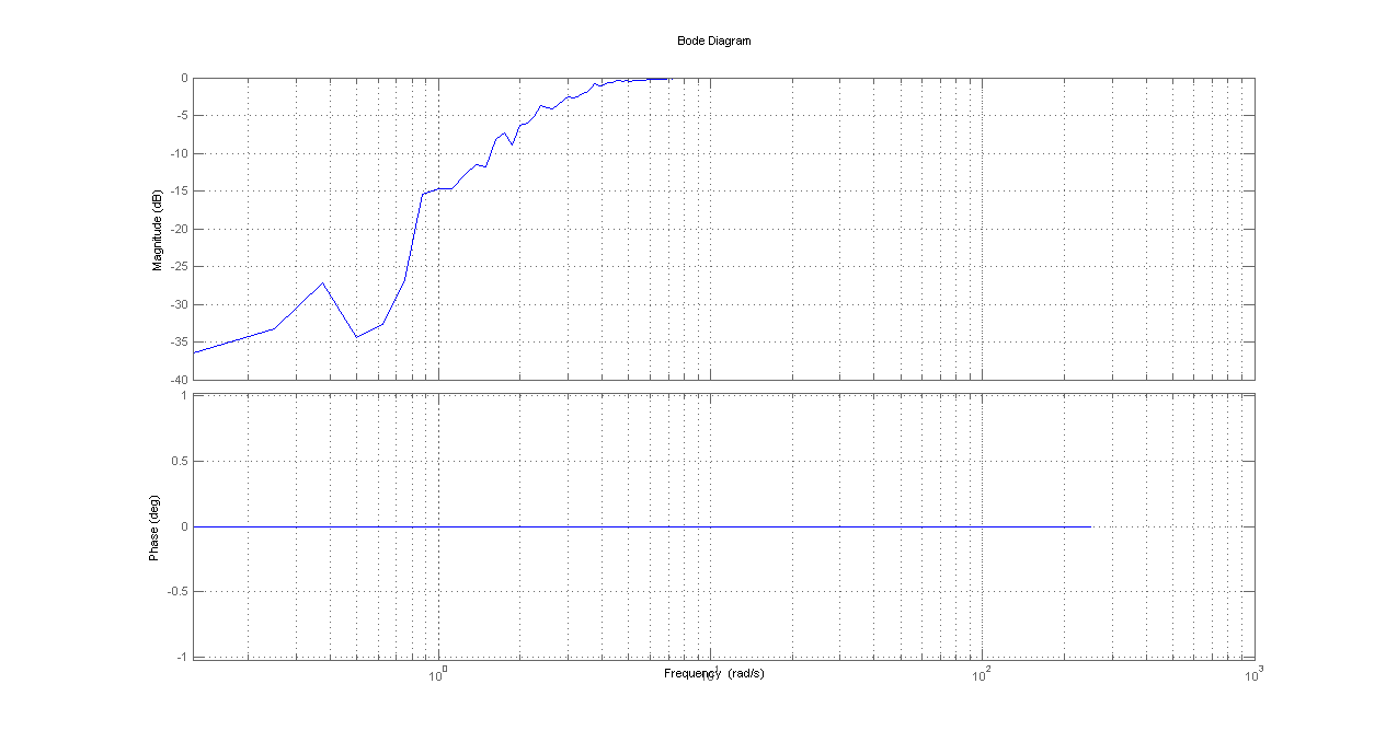
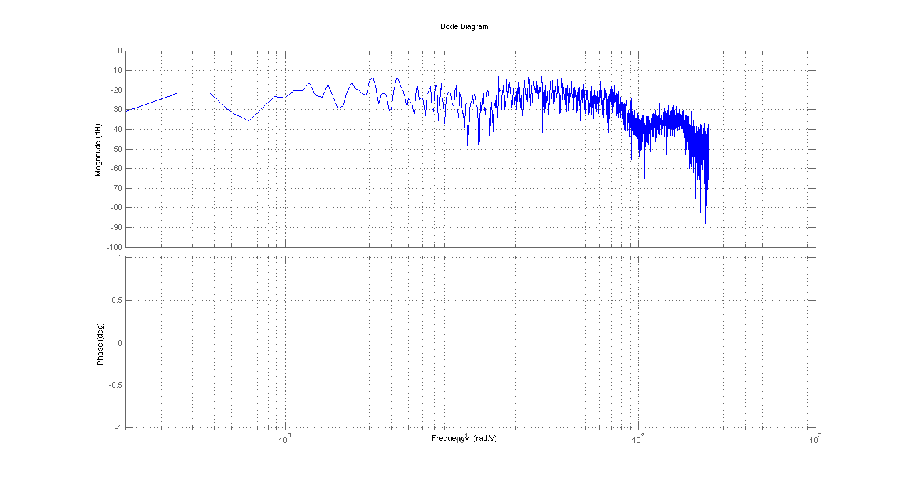
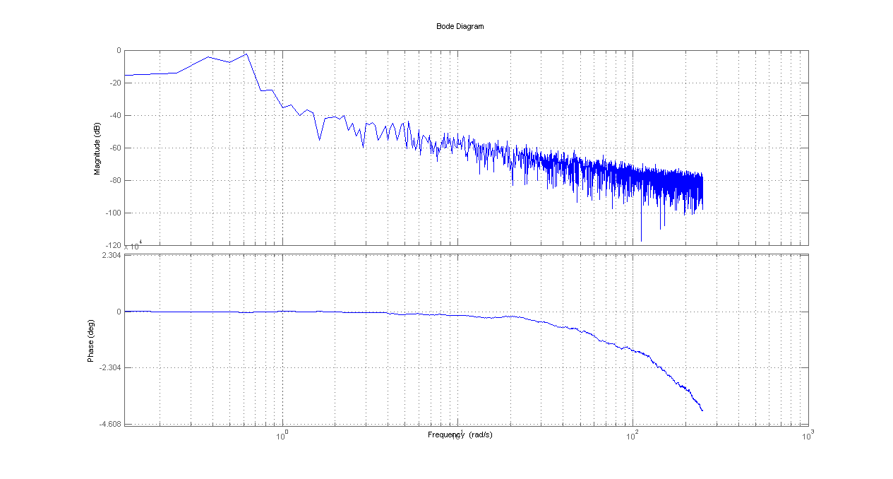
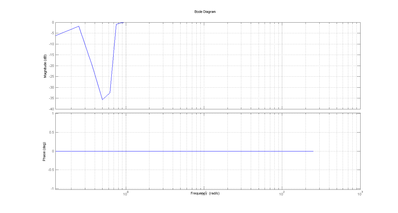
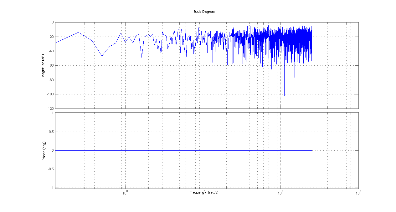
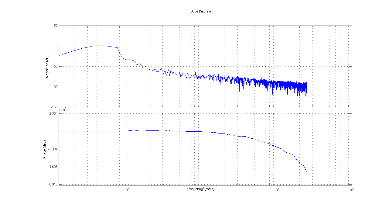
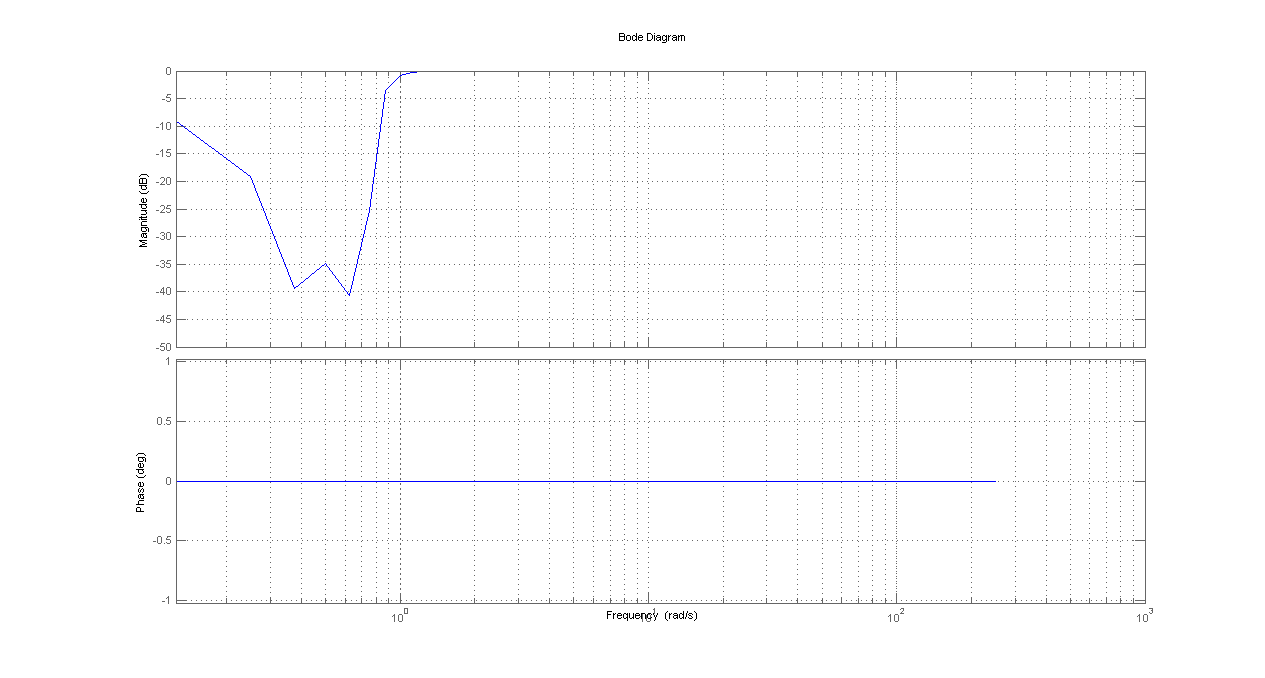
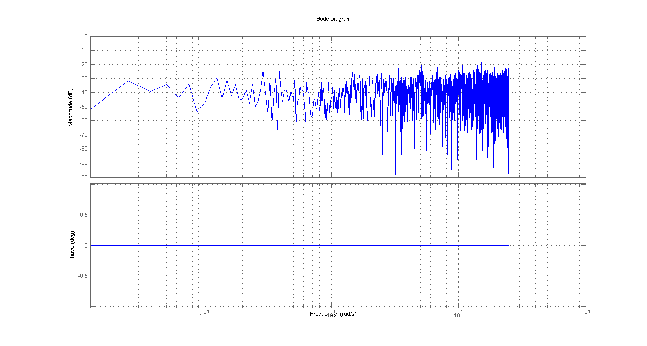
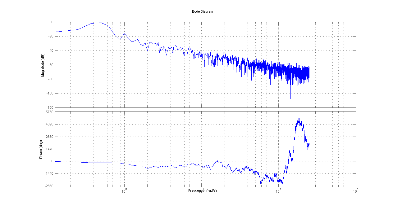
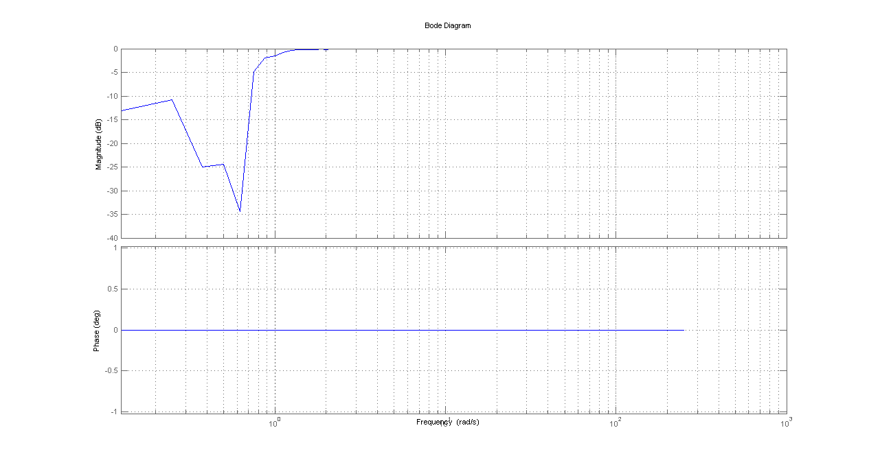
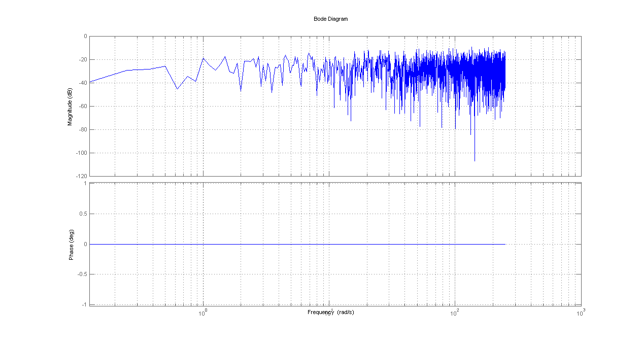
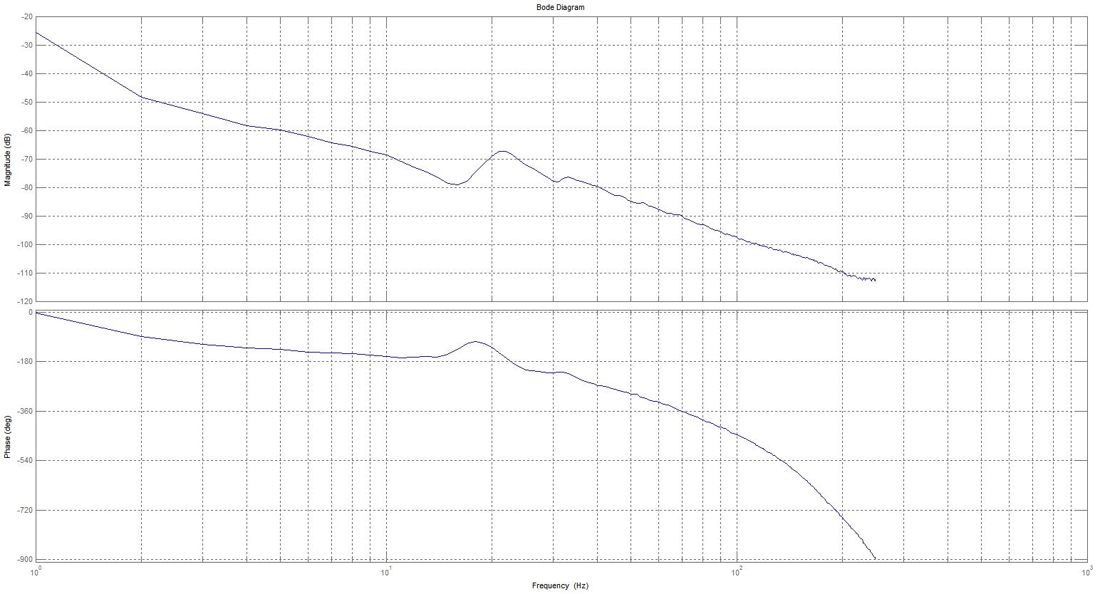
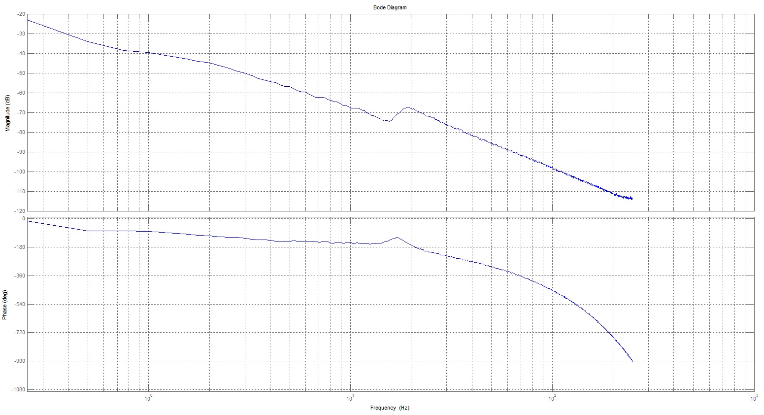
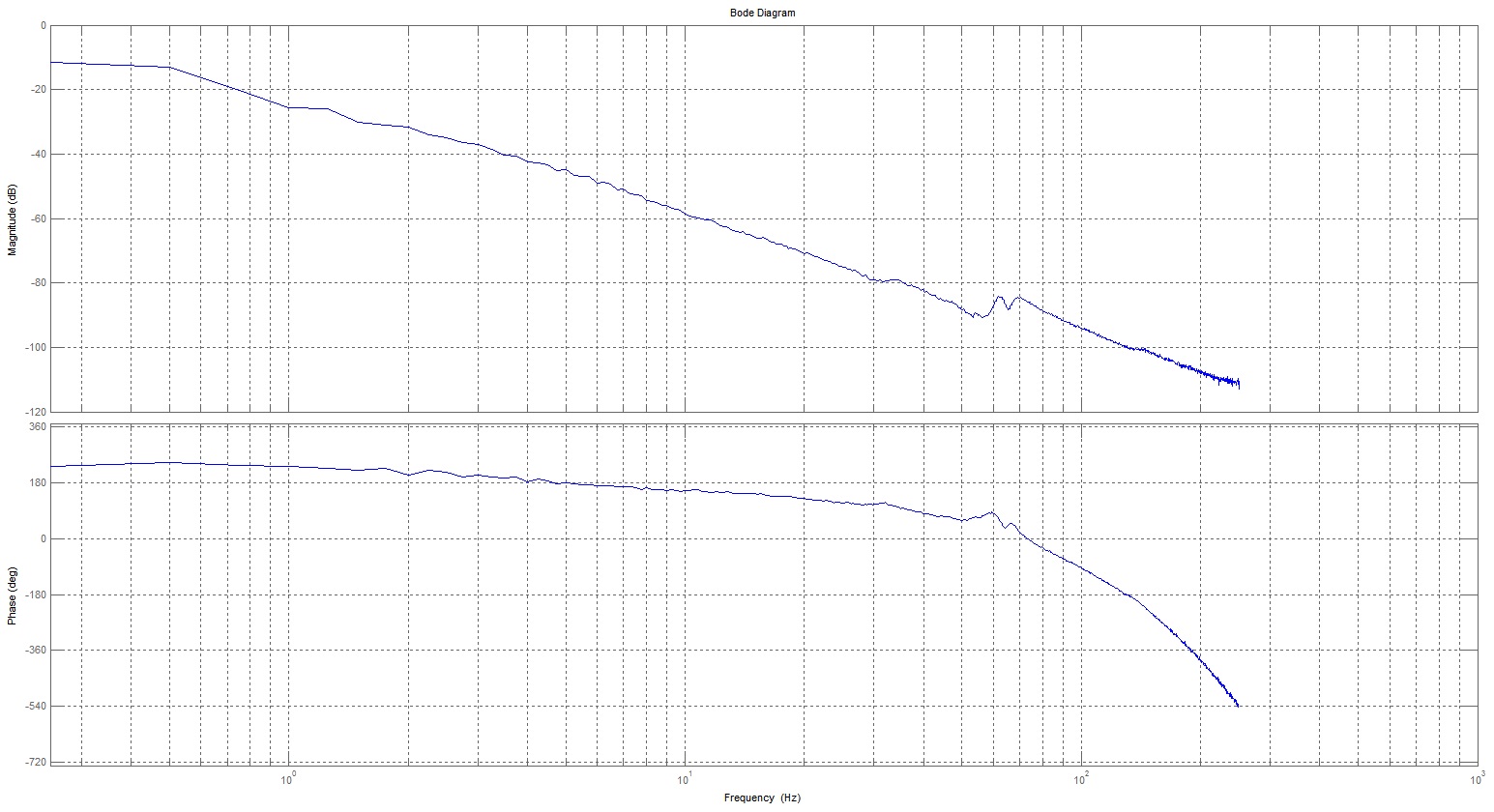
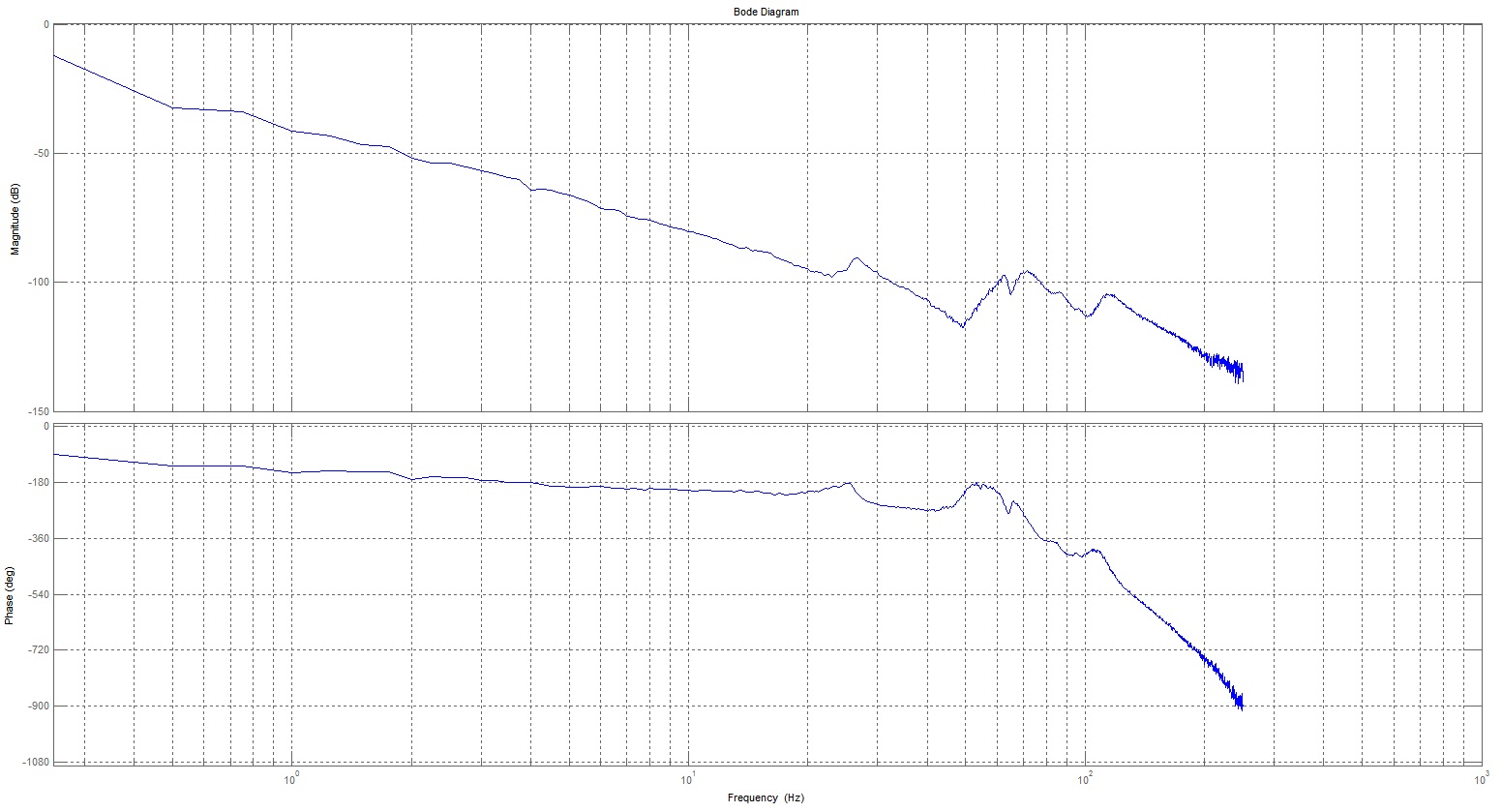
| As our initial plan states, we scheduled to do our FRF measurements by closing the loop with negative feedback on each axis, thus stabilizing it (with a low bandwidth controller), and then estimating the frequency response by using the three-point FRF method. We were able to get an acceptable FRF on the first axis (the vertical movement), however on the other three axes our results were unsatisfactory, with the main problem being the high noise making the gain and phase estimations unclear. |
| In order to rectify these unclear readings, we attempted to perform open-loop FRF measurements. These experiments were done with special care, as the axes should not be allowed to touch the airbags. The results were satisfactory to a high degree. |
 |
 |
 |
 |
Week 3: Mar 4 - Mar 10
| Improve the results of FRF measurements by applying new parametric identification methods |
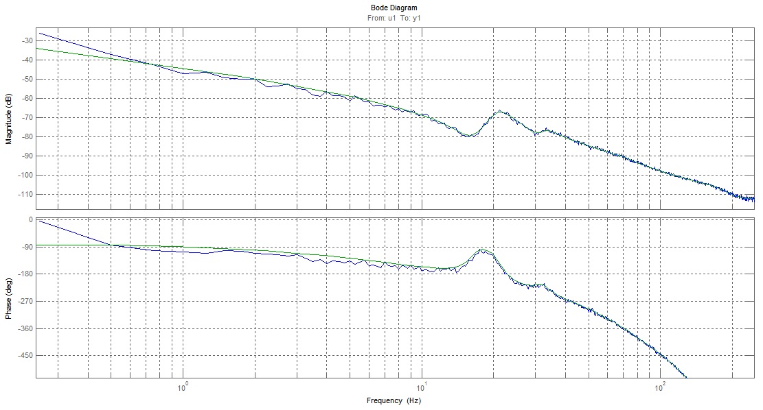
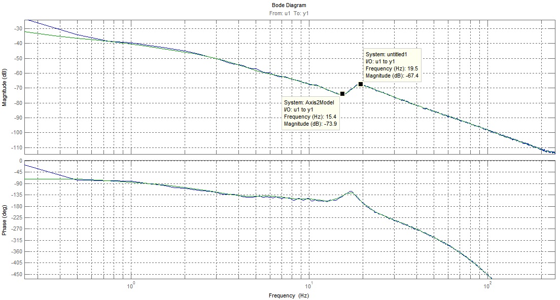
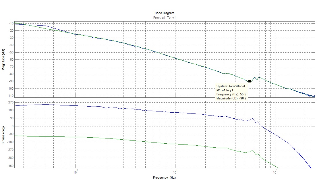
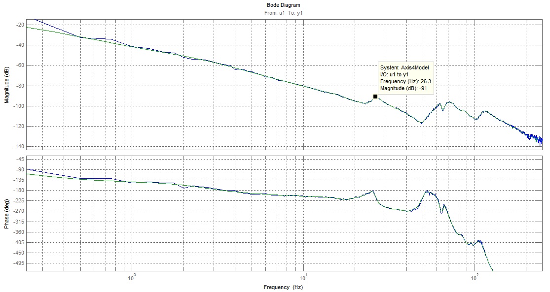
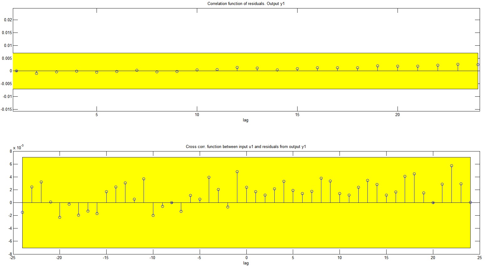
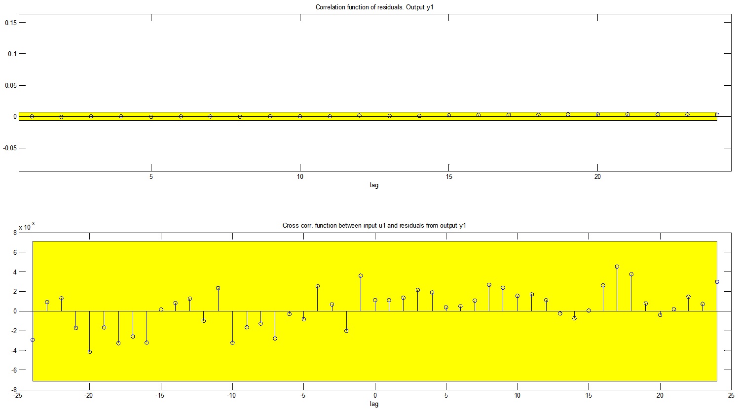
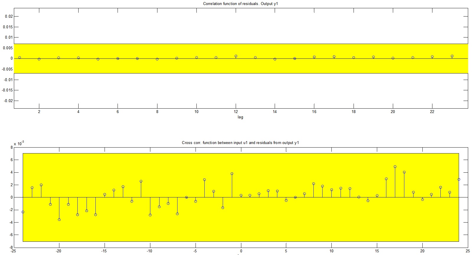
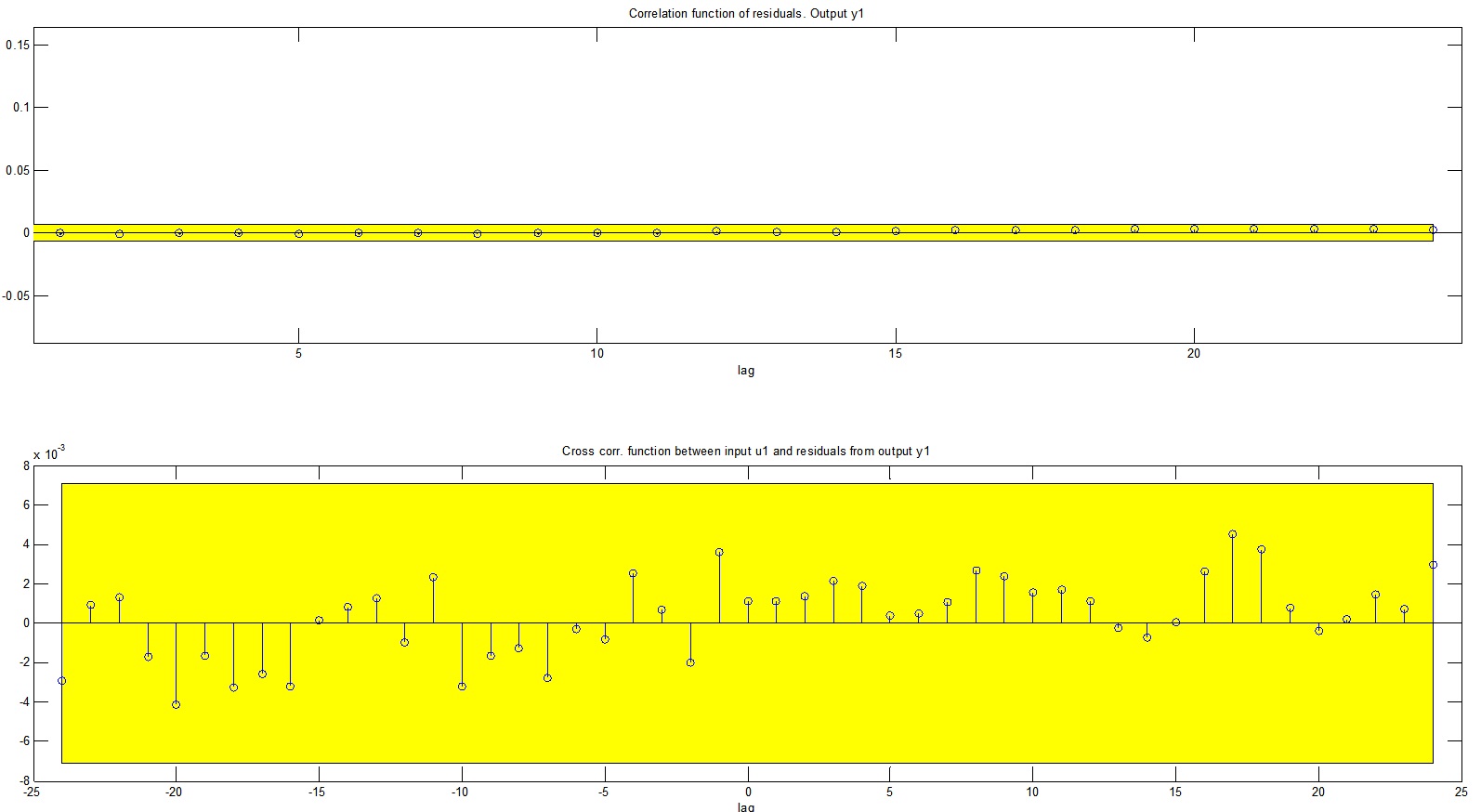
| In order to obtain high quality models for control design we proceeded to fit our frequency response data to discrete transfer functions using the System Identification Toolbox (using mainly the ARX and Box-Jenkins models). These high-order models were used for building our controllers. The advantage of using models is being able to observe our estimated performance (such as step responses) as well and not just stability margins (gain margin, phase margin, modulus margin etc.).
High-order models were used in order to catch all the dynamics and phase loss due to sampling the system shows. The first axis was fitted into a Box-Jenkins model of 30th order (30 coefficients for model numerator and denominator each, and another 30 coefficients for the noise model). The 2nd and 3rd axes were fitted into ARX models of 120th order (120 coefficients for A(q) and another 120 coefficients for B(q)). The 4th axis was fitted into a Box-Jenkins model of 60th order (60 coefficients for model numerator and denominator each, and another 60 coefficients for the noise model).
|
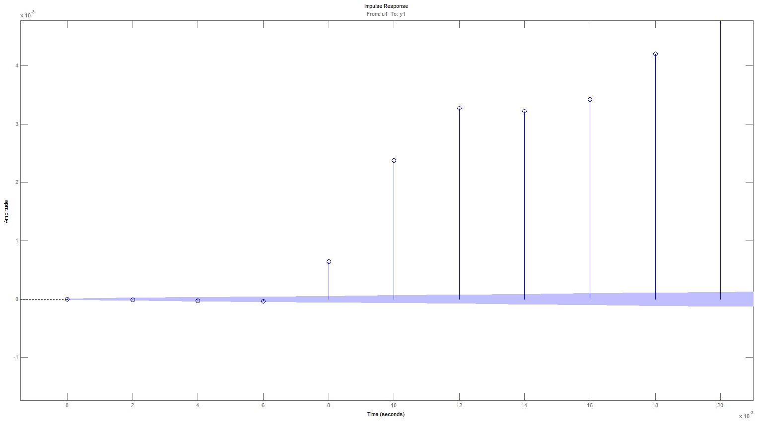
| Below we see a figure of the impulse response of the 4th Axis. We notice there is a 4 sample delay on our system. |
 |
 |
 |
 |
 |
 |
 |
 |
 |
Week 4: Mar 11 - Mar 17
| Controller Synthesis
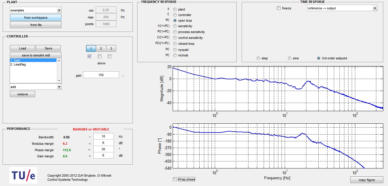
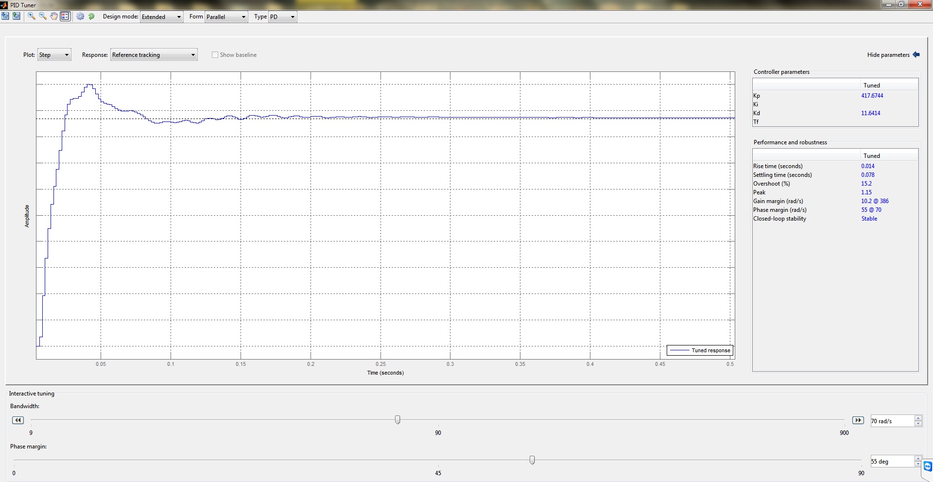
Using our previous system identification findings, we proceeded to our controller synthesis procedure. The parametric models allowed us to nicely observe the step response of our plant(s), and thus determine various performance and stability margins for our controllers (like Gain Margin, Phase Margin, Modulus Margin, Bandwidth, Settling time, Rise Time and Overshoot). The main tools we used were the loopshaping tool Shapeit and the PID tuning tool of Matlab. The complexity of the controllers was kept low, since our plants were not extremely complicated (resembled the expected double integrator transfer function quite substantially). |
| Below we see screenshots of the tools we used to synthesize our controllers. The PID tuning tool of Matlab offers automated synthesis, given the type, phase margin and bandwidth of the controller one chooses to design, but at the expense of limited controller order. Below we see ShapeIt, which while not automated, offers greater controller complexity to experiment with. |
 |
 |
| Below we can see our controllers' stability margins and performance properties. |
 |
Controller testing
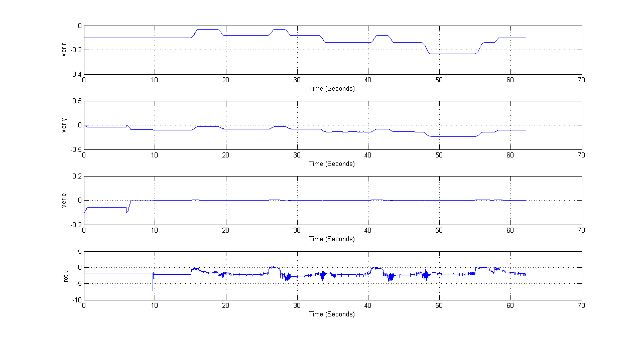
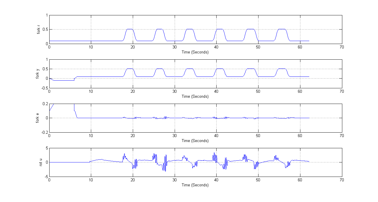
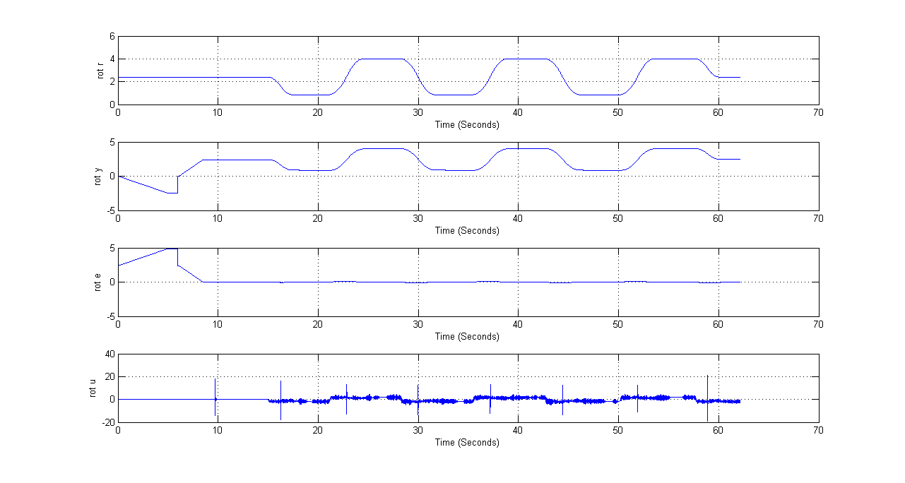
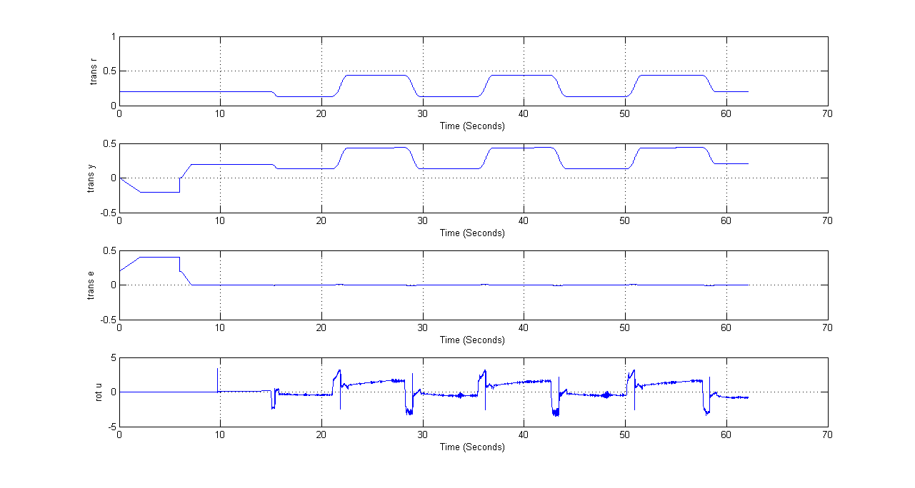
Having designed first controllers, we implemented them in the simulink model and tested their performance on the trajectory designed in the previous weeks. We started from "slow" trajectory, which took about one minute in total. Robot was moving without pizzas at this point. These tests gave us good overview on controller behavior as well as further trajectory improvements. Of course robot behavior on the trajectory is one of the most important specs of the controller design. Therefore controller synthesis and controller testing on the trajectory became an iterative procedure. By shortening the trajectory time (which made it more difficult to follow) we could give higher demands to the controllers.
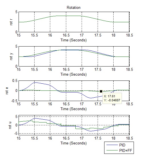
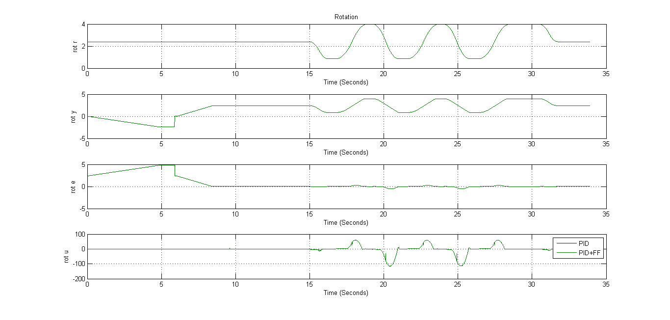
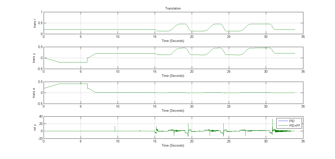
Below we presents four plots which were used to precisely observe behavior of four robot joints while following the trajectory. The plots correspond to vertical fork displacement, horizontal fork displacement, rotation and translation (from up-left to down-right). On each plot we can see: given trajectory, trajectory followed by the robot joint, error (difference of the first two plots), controller output (from the top to the bottom).
 |
 |
 |
 |
Trajectory improvements
The trajectory built in the previous weeks was changed. During initial testing it could be seen that the rotation of the robot took more time than changing height or translating. Thus changing the height during the rotation from the left to the right position did not result in a slower trajectory. The order of placing the pizza's was then changed, to create more space when putting down the pizza's. The trajectory was adjusted to place the pizzas in the following order: L2->R4->L3->R3->L4->R2. This resulted in more movement space when putting down the pizza's.
Week 5: Mar 18 - Mar 24
| - Improve controllers by adding feed forward. Construct low bandwidth controller, challenging trajectory to get a usable error profile to tune feed forward. | |||
| - After testing the new trajectory, the results were satisfactory. We were now able to pick and place pizza's succesfully at a low speed. The accelerations of the different movements were increased until the error would become to big. To further improve the trajectory, unnecessary motions were deleted. The retracting of the arm after putting down a pizza was deleted, because there was enough movement space inbetween the two shelves. This resulted in a considerable time gain. | |||
| - Consideration of different controller synthesis methods: Out of the various options we had to work with, PID tuning was the one that everyone had experience with, and thus contribute to the team. Additionally, other controller synthesis methods were discarded for various reasons, like unnecessary (H infinity robust control), hard to implement (Model Predictive Control), or focusing on different aspects instead of accuracy (LQR state space control).
| |||
|
Max. original error: 0.4001
|
Week 6: Mar 25 - Mar 31
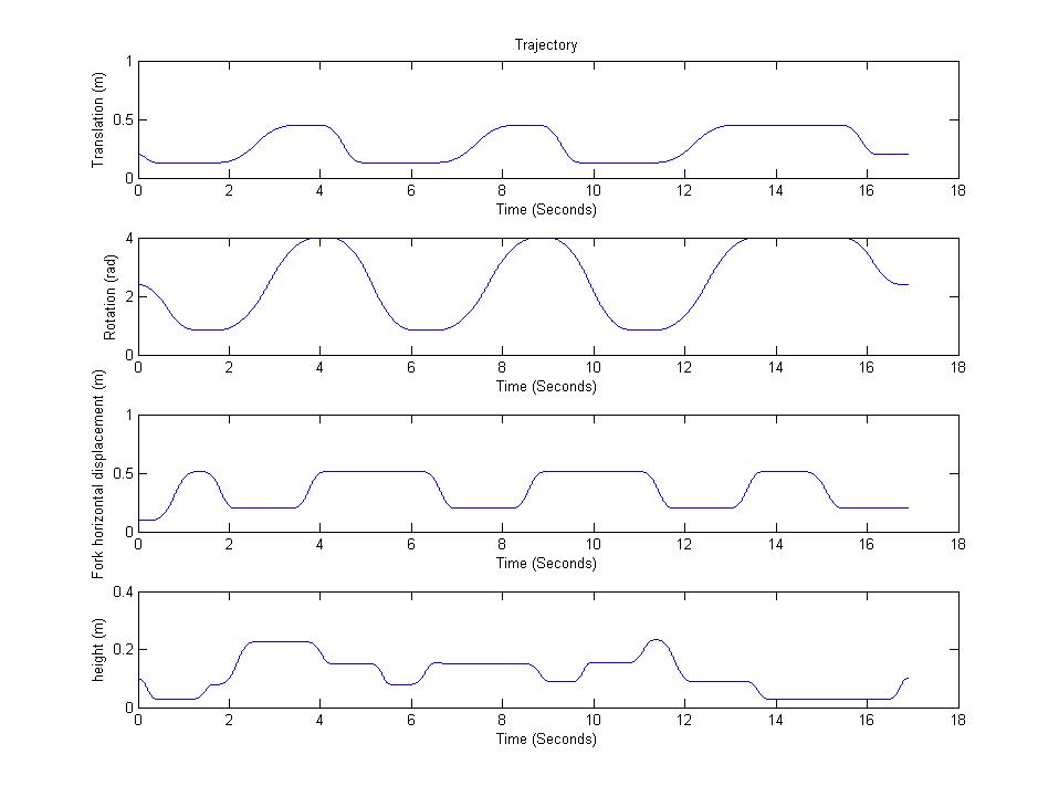
The next improvement for the trajectory was the overlap of movements. Until now, the movement in different directions was seperated as much as possible. However, it was noticed that this was not necesarry. For example, when putting down a pizza, instead of moving the fork out, then going down and then retracting the fork, these movements were combined. We achieved as much as 50% overlap while still placing the pizza's succesfully. This resulted in considerable trajection time reduction. The final trajectory is shown below.
 |
Week 7: Apr 1 - Apr 5
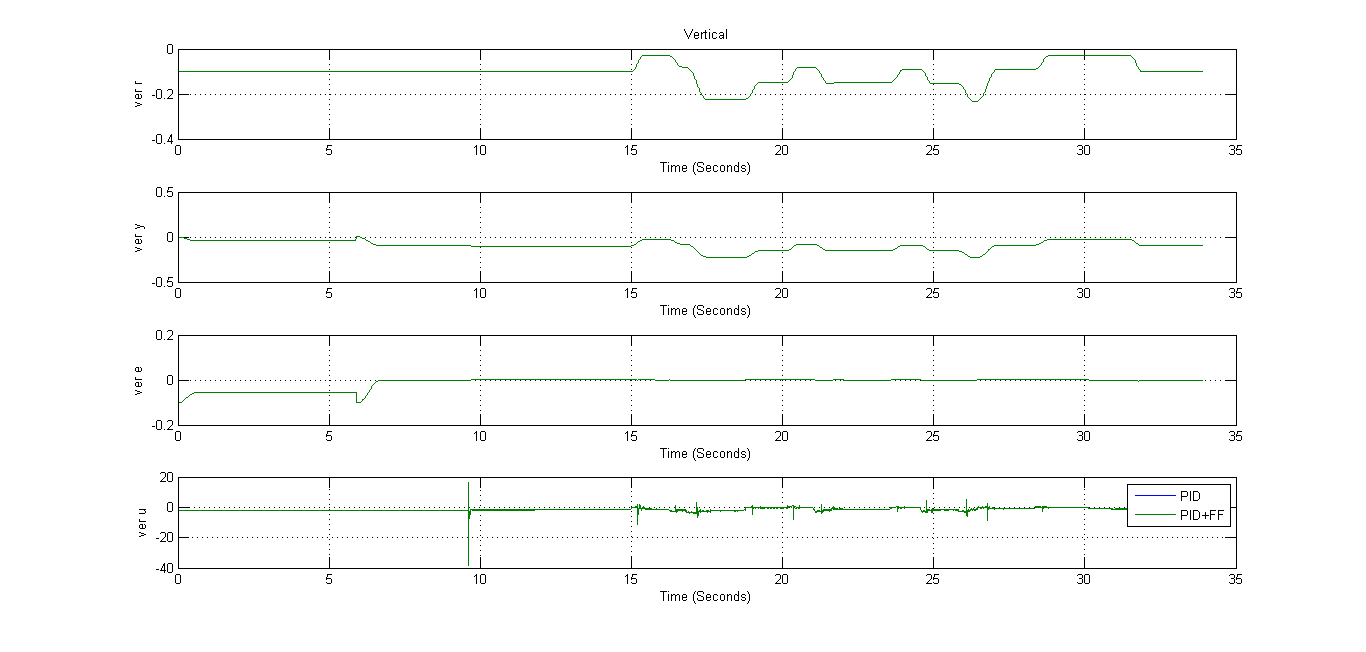
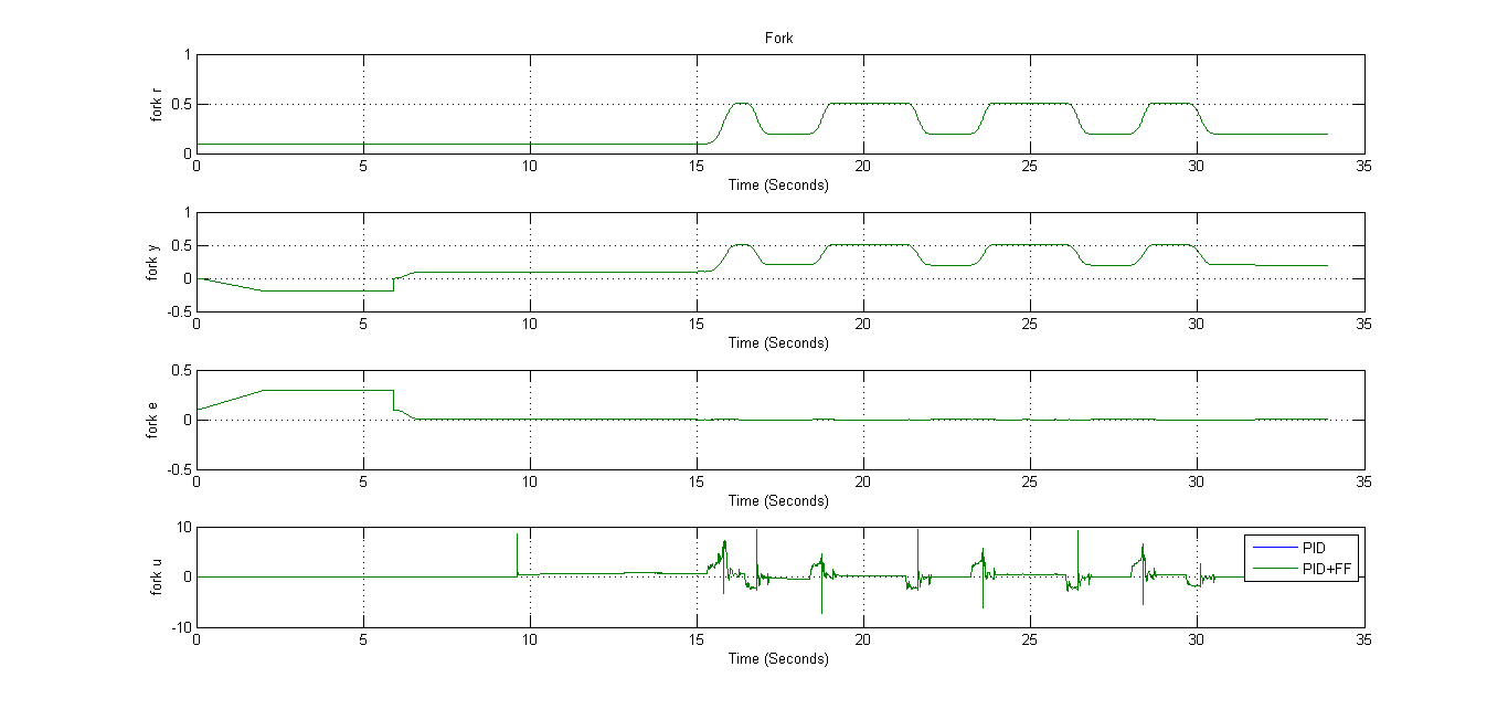
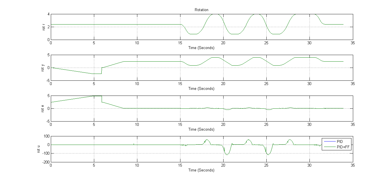
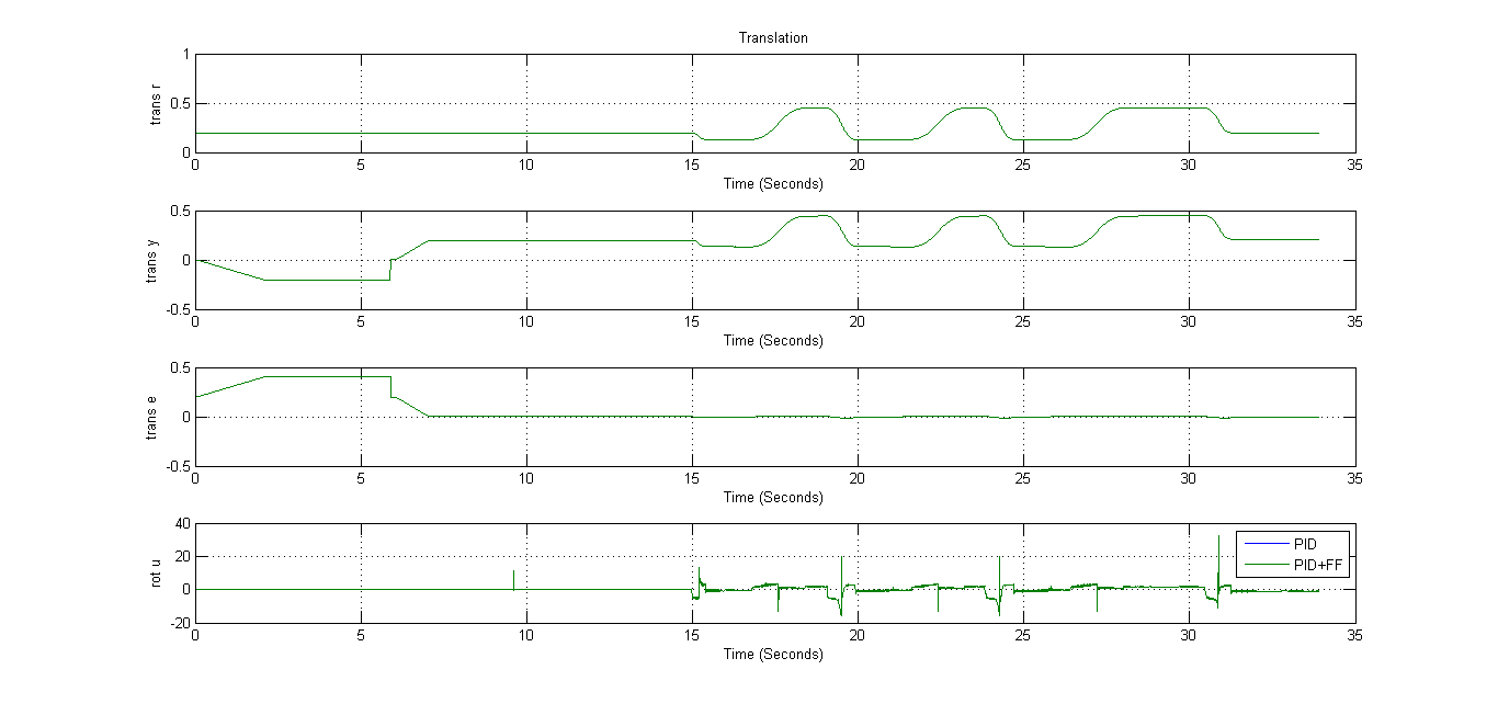
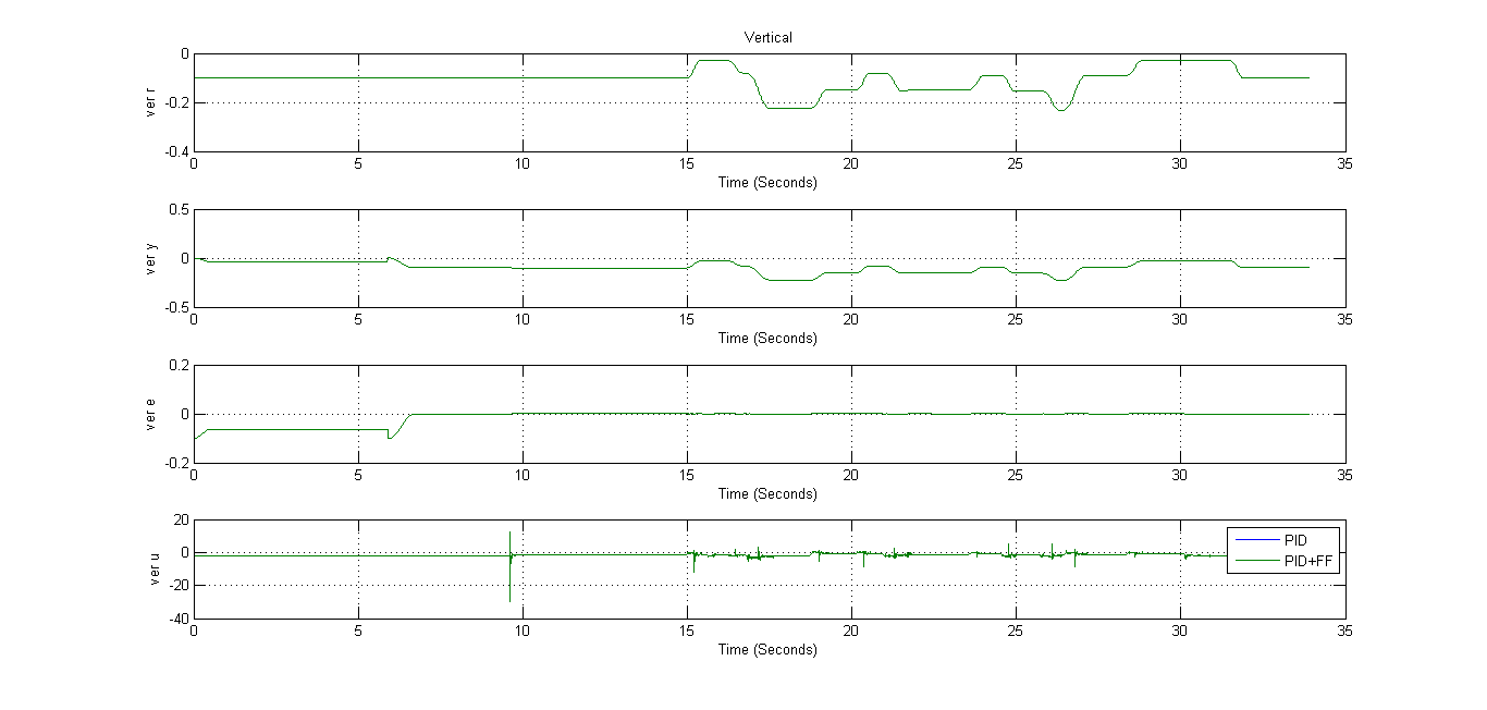
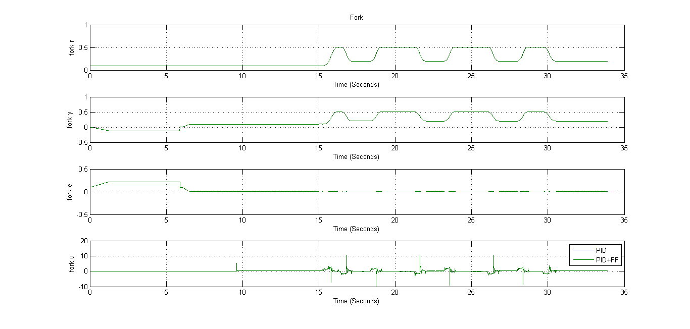
| This last week has been used for revision of the project, final adjustments and to test the overall result on the right robot. Up to this week all the tests have been performed on the left robot. With the controllers we have used until now we achieved as well a good performance on the right robot. Final results for both robots can be observed in the following plots. As stated before, the plots correspond to vertical fork displacement, horizontal fork displacement, rotation and translation (from up-left to down-right). On each plot we can see: given trajectory, trajectory followed by the robot joint, error (difference of the first two plots), controller output (from the top to the bottom).
|
| Left Robot |
 |
 |
 |
 |
Right Robot
 |
 |
 |
 |
